主要分析 Sigmoid 和 Softmax 对于二分类问题,二者之间的差异性.
曾涉及到 Sigmoid 和 Softmax 的问题一般用于交叉熵损失函数,如:
[1] - 机器学习 - 交叉熵Cross Entropy
[2] - CaffeLoss - SigmoidCrossEntropyLoss 推导与Python实现
[3] - Focal Loss 论文理解及公式推导
习惯性的认为,SigmoidCrossEntropyLoss 用于二类问题;SoftmaxCrossEntropyLoss 用于多类问题. 但,在二分类情况时,SoftmaxCrossEntropyLoss 与 SigmoidCrossEntropyLoss 作用等价.
这里从两方面分析下,对于 Sigmoid 和 Softmax 在二分类情况下的等价性.
主要参考 - ypwhs/sigmoid_and_softmax.ipynb.
1. 理论分析
二分类场景,
[1] - Sigmoid:
$$ \begin{equation} \begin{cases} p(y=1|x) = \frac{1}{1 + e ^{-\theta ^ T x}} \\ p(y=0|x) = 1 - p(y=1|x) = \frac{e ^{-\theta ^ T x}}{1 + e ^{-\theta ^ T x}} \end{cases} \end{equation} $$
[2] - Softmax:
$$ \begin{equation} \begin{cases} p(y=0|x) = \frac{e ^{\theta _0^T x} }{e ^{\theta _0^T x} + e ^{\theta _1^T x} } = \frac{e ^{(\theta _0^T - \theta _1^T)x} }{1 + e ^{(\theta _0^T - \theta _1^T) x} } \\ p(y=1|x) = 1 - p(y=0|x) \end{cases} \end{equation} $$
令 $\beta = -(\theta_0^T - \theta _1^T)$,则有:
$$ \begin{equation} \begin{cases} p(y=1|x) = \frac{1}{1 + e ^{-\beta ^ T x}} \\ p(y=0|x) = \frac{e ^{-\beta ^ T x}}{1 + e ^{-\beta ^ T x}} \end{cases} \end{equation} $$
可见,此时,Softmax 与 Sigmoid 二者理论公式的等价性.
2. 基于 Kera 的计算对比
以猫狗分类的数据集为例,采用在 ImageNet 上与训练的 Xception 模型导出的特征.( 复制于 ypwhs/sigmoid_and_softmax.ipynb 中的代码. )
gap_Xception.h5
import h5py
import numpy as np
from sklearn.model_selection import train_test_split

from keras.layers import *
from keras.models import *
from keras.optimizers import *
from keras.utils import to_categorical

import matplotlib.pyplot as plt

np.random.seed(20180520)

#---------------------------------
#      加载猫狗分类的特征数据
#---------------------------------
with h5py.File("gap_Xception.h5", 'r') as h:
    X = np.array(h['train'])
    y = np.array(h['label'])

X_train, X_test, y_train, y_test = train_test_split(X, y, test_size=0.2)

y_train_softmax = to_categorical(y_train) # ont-hot
y_test_softmax = to_categorical(y_test)


#---------------------------------
#           Softmax
#---------------------------------
# loss: Softmax Cross Entropy Loss
input_tensor = Input(X.shape[1:])
x = input_tensor
x = Dropout(0.5)(x)
softmax = Dense(2, activation='softmax')
x = softmax(x)
model = Model(input_tensor, x)
model.compile(optimizer=SGD(1e-3),  # lr = 1e-3
              loss='categorical_crossentropy',
              metrics=['accuracy'])

softmax_weights, softmax_bias = softmax.get_weights()

history_softmax = model.fit(X_train, y_train_softmax, batch_size=128, epochs=5,
                            validation_data=(X_test, y_test_softmax))

#---------------------------------
#           Sigmoid
#---------------------------------
# loss: Binary(Sigmoid) Cross Entropy Loss
np.random.seed(20180520)
input_tensor = Input(X.shape[1:])
x = input_tensor
x = Dropout(0.5)(x)
sigmoid = Dense(1, activation='sigmoid')
x = sigmoid(x)
model = Model(input_tensor, x)
model.compile(optimizer=SGD(2e-3),  # lr = 2e-3
              loss='binary_crossentropy',
              metrics=['accuracy'])

# Sigmoid 权重初始化为 Softmax 的权重计算差值
# beta = sigmoid weights
beta = -(softmax_weights[:,0] - softmax_weights[:,1]).reshape((-1, 1))

sigmoid.set_weights([beta, np.zeros(1)]) # set beta to sigmoid weights

history_sigmoid = model.fit(X_train, y_train, batch_size=128, epochs=5, validation_data=(X_test, y_test))


#---------------------------------
#           Sigmoid
#---------------------------------
input_tensor = Input(X.shape[1:])
x = input_tensor
x = Dropout(0.5)(x)
sigmoid = Dense(1, activation='sigmoid')
x = sigmoid(x)
model = Model(input_tensor, x)
model.compile(optimizer=SGD(2e-3),  # lr = 2e-3
              loss='binary_crossentropy',
              metrics=['accuracy'])

# random init Sigmoid weights
# 随机初始化 Sigmoid 权重
history_sigmoid_2 = model.fit(X_train, y_train, batch_size=128, epochs=5, validation_data=(X_test, y_test))
训练过程输出:
Softmax:
Train on 20000 samples, validate on 5000 samples
Epoch 1/5
20000/20000 [==============================] - 1s 68us/step - loss: 0.4711 - acc: 0.8535 - val_loss: 0.3765 - val_acc: 0.9642
Epoch 2/5
20000/20000 [==============================] - 0s 13us/step - loss: 0.3338 - acc: 0.9486 - val_loss: 0.2825 - val_acc: 0.9816
Epoch 3/5
20000/20000 [==============================] - 0s 11us/step - loss: 0.2594 - acc: 0.9726 - val_loss: 0.2279 - val_acc: 0.9858
Epoch 4/5
20000/20000 [==============================] - 0s 11us/step - loss: 0.2160 - acc: 0.9799 - val_loss: 0.1923 - val_acc: 0.9866
Epoch 5/5
20000/20000 [==============================] - 0s 13us/step - loss: 0.1860 - acc: 0.9825 - val_loss: 0.1677 - val_acc: 0.9868
Sigmoid With Softmax Weights:
Train on 20000 samples, validate on 5000 samples
Epoch 1/5
20000/20000 [==============================] - 0s 18us/step - loss: 0.4706 - acc: 0.8544 - val_loss: 0.3766 - val_acc: 0.9644
Epoch 2/5
20000/20000 [==============================] - 0s 12us/step - loss: 0.3346 - acc: 0.9476 - val_loss: 0.2824 - val_acc: 0.9816
Epoch 3/5
20000/20000 [==============================] - 0s 14us/step - loss: 0.2613 - acc: 0.9709 - val_loss: 0.2275 - val_acc: 0.9860
Epoch 4/5
20000/20000 [==============================] - 0s 14us/step - loss: 0.2151 - acc: 0.9789 - val_loss: 0.1923 - val_acc: 0.9868
Epoch 5/5
20000/20000 [==============================] - 0s 11us/step - loss: 0.1857 - acc: 0.9825 - val_loss: 0.1676 - val_acc: 0.9872
Sigmoid With Random Init Weight:
Train on 20000 samples, validate on 5000 samples
Epoch 1/5
20000/20000 [==============================] - 0s 18us/step - loss: 0.5690 - acc: 0.7607 - val_loss: 0.4415 - val_acc: 0.9718
Epoch 2/5
20000/20000 [==============================] - 0s 11us/step - loss: 0.3753 - acc: 0.9576 - val_loss: 0.3151 - val_acc: 0.9852
Epoch 3/5
20000/20000 [==============================] - 0s 12us/step - loss: 0.2819 - acc: 0.9814 - val_loss: 0.2464 - val_acc: 0.9878
Epoch 4/5
20000/20000 [==============================] - 0s 12us/step - loss: 0.2267 - acc: 0.9858 - val_loss: 0.2042 - val_acc: 0.9882
Epoch 5/5
20000/20000 [==============================] - 0s 11us/step - loss: 0.1921 - acc: 0.9872 - val_loss: 0.1759 - val_acc: 0.9882
2.1 训练 loss 曲线变化情况对比
plt.plot(history_sigmoid.history['loss'])
plt.plot(history_softmax.history['loss'])

plt.plot(history_sigmoid.history['val_loss'])
plt.plot(history_softmax.history['val_loss'])

plt.ylabel('loss')
plt.xlabel('epoch')

plt.legend(['sigmoid_loss', 'softmax_loss',
            'sigmoid_val_loss', 'softmax_val_loss'], loc='upper right')
plt.show()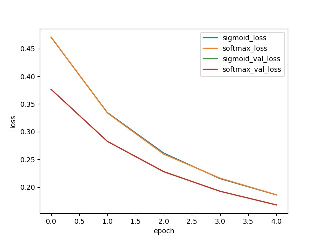
从图中可知,Sigmoid 和 Softmax 的训练曲线几乎完全重合.
2.2 Loss 差值可视化对比
plt.plot(np.array(history_sigmoid.history['val_loss']) - np.array(history_softmax.history['val_loss']))
plt.plot(np.array(history_sigmoid.history['val_loss']) - np.array(history_sigmoid_2.history['val_loss']))

plt.ylabel('loss')
plt.xlabel('epoch')

plt.legend(['sigmoid_softmax_beta_gap', 'sigmoid_random_weight_gap'], loc='upper right')
plt.show()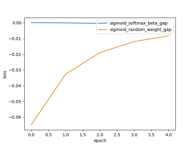
图中蓝色曲线几乎一直是 0,其表示 Sigmoid 和 Softmax 训练的模型的 loss 差异性很小. 但黄色曲线 的差值相对就较大,其采用的随机初始化 Sigmoid 权重值,影响了训练过程中的 loss 曲线的变化.
也就是说,如果设置了正确的 beta 值,Sigmoid 与 Softmax 的效果可认为时等价的.
2.3 总结
对于二分类问题,
[1] - Sigmoid 与 Softmax 完全等价.
[2] - Sigmoid 与 Softmax 分类器的权值可以相互转换.
[3] - Softmax 的学习率是 Sigmoid 学习率的2倍. (如:1e-3与2e-3)
[4] - Softmax 会比 Sigmoid 浪费 2 倍的权值空间(权重参数是两倍).
5 条评论
请问二分类下,sigmoid = Dense(1, activation='sigmoid') 和softmax = Dense(2, activation='softmax') 用哪一个是不是都是一样的呢?
效果一致,但权重参数量会不一致.
为什么学习率需要两倍呢,有推导吗
二分类的情况下θ_1 = 1-θ_0, 那么β=1-2θ_0, 所以就是两倍的关系
不好意思没有推导,是炼丹经验吧