迁移学习教程 - cs231n Notes - Transfer Learning
一般情况下,当数据量较少时,不会完全重新从头开始训练 CNN 网络(权重随机初始化). 通常会采用在大规模数据集,如ImageNet,预训练的 ConvNet 模型权重,作为网络训练的舒适化;或者,用作特征提取器.
迁移学习的两种主要应用场景:
[1] - Finetuning the convnet
相比于随机初始化网络,采用预训练的模型作为网络初始化.
[2] - ConvNet 作为特征提取器
除了网络的最后一层全连接层,冻结网络其它层的权重. 将最后一层全连接层替换为新的权重随机初始化的全连接层,且只训练新的全连接层.
1. 数据加载
采用 torchvision 和 torch.utils.data进行数据加载.
这里以 ants蚂蚁 和 bees蜜蜂 的分类模型训练为例.
数据集中每个类别分别有 120 张训练图像,75 张验证图像. (数据集非常小.)
ants && bees 数据集
数据加载与数据增强实现:
# Data augmentation and normalization for training
# Just normalization for validation
data_transforms = {
    'train': transforms.Compose([
        transforms.RandomResizedCrop(224),
        transforms.RandomHorizontalFlip(),
        transforms.ToTensor(),
        transforms.Normalize([0.485, 0.456, 0.406], [0.229, 0.224, 0.225])
    ]),
    'val': transforms.Compose([
        transforms.Resize(256),
        transforms.CenterCrop(224),
        transforms.ToTensor(),
        transforms.Normalize([0.485, 0.456, 0.406], [0.229, 0.224, 0.225])
    ]),
}

data_dir = './datas/hymenoptera'
image_datasets = {x: datasets.ImageFolder(os.path.join(data_dir, x),
                                          data_transforms[x])
                  for x in ['train', 'val']}
dataloaders = {x: torch.utils.data.DataLoader(image_datasets[x], batch_size=4,
                                             shuffle=True, num_workers=4)
              for x in ['train', 'val']}
dataset_sizes = {x: len(image_datasets[x]) for x in ['train', 'val']}
class_names = image_datasets['train'].classes

device = torch.device("cuda:0" if torch.cuda.is_available() else "cpu")
部分图像可视化:
# Vis images
def imshow(inp, title=None):
    """Imshow for Tensor."""
    inp = inp.numpy().transpose((1, 2, 0))
    mean = np.array([0.485, 0.456, 0.406])
    std = np.array([0.229, 0.224, 0.225])
    inp = std * inp + mean
    inp = np.clip(inp, 0, 1)
    plt.imshow(inp)
    if title is not None:
        plt.title(title)
    plt.pause(0.001)

# Get a batch of training data
inputs, classes = next(iter(dataloaders['train']))

# Make a grid from batch
out = torchvision.utils.make_grid(inputs)
imshow(out, title=[class_names[x] for x in classes])
如:
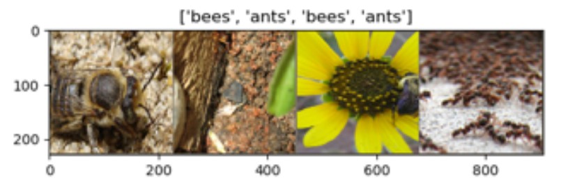
2. 模型训练
模型训练的相关函数,如:
- Scheduling the learning rate
- Saving the best model
def train_model(model, criterion, optimizer, scheduler, num_epochs=25):
since = time.time()
best_model_wts = copy.deepcopy(model.state_dict())
best_acc = 0.0
for epoch in range(num_epochs):
print('Epoch {}/{}'.format(epoch, num_epochs - 1))
print('-' * 10)
# 每个 epoch 包含 training 和 validation phase.
for phase in ['train', 'val']:
if phase == 'train':
scheduler.step()
model.train() # Set model to training mode
else:
model.eval() # Set model to evaluate mode
running_loss = 0.0
running_corrects = 0
# Iterate over data.
for inputs, labels in dataloaders[phase]:
inputs = inputs.to(device)
labels = labels.to(device)
# zero the parameter gradients
optimizer.zero_grad()
# forward
# track history if only in train
with torch.set_grad_enabled(phase == 'train'):
outputs = model(inputs)
_, preds = torch.max(outputs, 1)
loss = criterion(outputs, labels)
# backward + optimize only if in training phase
if phase == 'train':
loss.backward()
optimizer.step()
# statistics
running_loss += loss.item() * inputs.size(0)
running_corrects += torch.sum(preds == labels.data)
epoch_loss = running_loss / dataset_sizes[phase]
epoch_acc = running_corrects.double() / dataset_sizes[phase]
print('{} Loss: {:.4f} Acc: {:.4f}'.format(
phase, epoch_loss, epoch_acc))
# deep copy the model
if phase == 'val' and epoch_acc > best_acc:
best_acc = epoch_acc
best_model_wts = copy.deepcopy(model.state_dict())
print()
time_elapsed = time.time() - since
print('Training complete in {:.0f}m {:.0f}s'.format(
time_elapsed // 60, time_elapsed % 60))
print('Best val Acc: {:4f}'.format(best_acc))
# load best model weights
model.load_state_dict(best_model_wts)
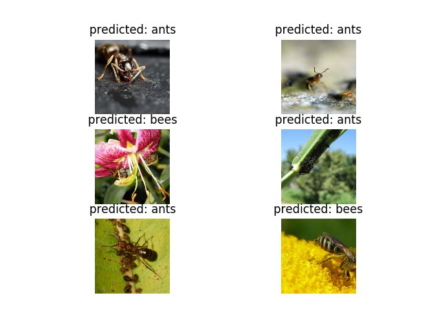
return model3. 模型预测可视化
# Visualizing the model predictions
def visualize_model(model, num_images=6):
    was_training = model.training
    model.eval()
    images_so_far = 0
    fig = plt.figure()

    with torch.no_grad():
        for i, (inputs, labels) in enumerate(dataloaders['val']):
            inputs = inputs.to(device)
            labels = labels.to(device)

            outputs = model(inputs)
            _, preds = torch.max(outputs, 1)

            for j in range(inputs.size()[0]):
                images_so_far += 1
                ax = plt.subplot(num_images//2, 2, images_so_far)
                ax.axis('off')
                ax.set_title('predicted: {}'.format(class_names[preds[j]]))
                imshow(inputs.cpu().data[j])

                if images_so_far == num_images:
                    model.train(mode=was_training)
                    return
        model.train(mode=was_training)
4. 模型 Finetune
# 网络 Finetuning
# 加载 torchvision 提供的预训练模型,并重置网络最后一个全连接层.

model_ft = models.resnet18(pretrained=True)
num_ftrs = model_ft.fc.in_features # 最后一层全连接层的输入 channels.
model_ft.fc = nn.Linear(num_ftrs, 2) # 重置最后一个全连接层.

model_ft = model_ft.to(device) # GPU CUDA 训练

criterion = nn.CrossEntropyLoss() # Loss 函数

#全部参数都是待优化参数.
optimizer_ft = optim.SGD(model_ft.parameters(), lr=0.001, momentum=0.9)

# 每 step_size=7 个 epochs, 以 0.1 的因子衰减 LR.
exp_lr_scheduler = lr_scheduler.StepLR(optimizer_ft, step_size=7, gamma=0.1)

# 模型 Train and evaluate
# CPU 上大概 15-25 分钟训练 25 个 epochs.
# GPU 上大概只需要 1 分钟左右.
model_ft = train_model(model_ft, criterion, optimizer_ft, exp_lr_scheduler,
                       num_epochs=25)
#
visualize_model(model_ft)
模型训练状态,如:
Epoch 0/24
----------
train Loss: 0.7185 Acc: 0.6352
val Loss: 0.1778 Acc: 0.9412

Epoch 1/24
----------
train Loss: 0.5723 Acc: 0.7705
val Loss: 0.3354 Acc: 0.8889

Epoch 2/24
----------
train Loss: 0.4694 Acc: 0.7787
val Loss: 0.3613 Acc: 0.8431

Epoch 3/24
----------
train Loss: 0.5598 Acc: 0.7787
val Loss: 0.3293 Acc: 0.8562

Epoch 4/24
----------
train Loss: 0.8370 Acc: 0.7254
val Loss: 0.4073 Acc: 0.8758

Epoch 5/24
----------
train Loss: 0.6716 Acc: 0.7664
val Loss: 0.3560 Acc: 0.8889

Epoch 6/24
----------
train Loss: 0.6657 Acc: 0.7582
val Loss: 0.6429 Acc: 0.8039

Epoch 7/24
----------
train Loss: 0.4766 Acc: 0.8279
val Loss: 0.2550 Acc: 0.9216

Epoch 8/24
----------
train Loss: 0.3360 Acc: 0.8811
val Loss: 0.2553 Acc: 0.8954

Epoch 9/24
----------
train Loss: 0.2963 Acc: 0.8607
val Loss: 0.3153 Acc: 0.8889

Epoch 10/24
----------
train Loss: 0.2896 Acc: 0.8934
val Loss: 0.2231 Acc: 0.9216

Epoch 11/24
----------
train Loss: 0.2963 Acc: 0.8852
val Loss: 0.2183 Acc: 0.9216

Epoch 12/24
----------
train Loss: 0.2992 Acc: 0.8811
val Loss: 0.2157 Acc: 0.9150

Epoch 13/24
----------
train Loss: 0.3763 Acc: 0.8402
val Loss: 0.2259 Acc: 0.9150

Epoch 14/24
----------
train Loss: 0.3455 Acc: 0.8648
val Loss: 0.2087 Acc: 0.9216

Epoch 15/24
----------
train Loss: 0.3301 Acc: 0.8361
val Loss: 0.2140 Acc: 0.9216

Epoch 16/24
----------
train Loss: 0.2579 Acc: 0.9057
val Loss: 0.2073 Acc: 0.9216

Epoch 17/24
----------
train Loss: 0.2737 Acc: 0.8852
val Loss: 0.1913 Acc: 0.9281

Epoch 18/24
----------
train Loss: 0.2700 Acc: 0.8770
val Loss: 0.2257 Acc: 0.9281

Epoch 19/24
----------
train Loss: 0.3633 Acc: 0.8361
val Loss: 0.1956 Acc: 0.9281

Epoch 20/24
----------
train Loss: 0.2900 Acc: 0.8648
val Loss: 0.2432 Acc: 0.8954

Epoch 21/24
----------
train Loss: 0.2780 Acc: 0.8730
val Loss: 0.1862 Acc: 0.9281

Epoch 22/24
----------
train Loss: 0.2875 Acc: 0.8730
val Loss: 0.1963 Acc: 0.9346

Epoch 23/24
----------
train Loss: 0.2838 Acc: 0.8811
val Loss: 0.2086 Acc: 0.9216

Epoch 24/24
----------
train Loss: 0.2458 Acc: 0.8852
val Loss: 0.2002 Acc: 0.9346

Training complete in 1m 13s
Best val Acc: 0.941176
模型预测结果可视化,如:
5. 特征提取器
采用网络作为特征提取器时,需要冻结网络所有的网络层,除了最后一个网络层. 采用 requires_grad==False 来冻结网络层参数,以使得在 backward() 时不计算网络层梯度.
Autograd mechanics
# 加载 torchvision.models 中的网络模型.
model_conv = torchvision.models.resnet18(pretrained=True)
for param in model_conv.parameters():
    param.requires_grad = False

# 默认只有新建的网络层模块的参数的 requires_grad=True
num_ftrs = model_conv.fc.in_features
model_conv.fc = nn.Linear(num_ftrs, 2)

model_conv = model_conv.to(device)

criterion = nn.CrossEntropyLoss()

# 只有最后一层网络层的参数是待优化参数.
optimizer_conv = optim.SGD(model_conv.fc.parameters(), lr=0.001, momentum=0.9)

# 每 step_size=7 个 epochs, 以 0.1 的因子衰减 LR.
exp_lr_scheduler = lr_scheduler.StepLR(optimizer_conv, step_size=7, gamma=0.1)


# 模型 Train 和 evaluate
# CPU 上的训练时间大概是 5-15 分钟训练 25 个 epochs.
# 因为网络中的大部分梯度不需要计算.
# 不过,forward前向计算是要进行计算的.
模型训练过程输出,如:
Epoch 0/24
----------
train Loss: 0.5825 Acc: 0.7336
val Loss: 0.3804 Acc: 0.8431
Epoch 1/24
----------
train Loss: 0.6608 Acc: 0.7131
val Loss: 0.1986 Acc: 0.9216
Epoch 2/24
----------
train Loss: 0.4897 Acc: 0.7951
val Loss: 0.1771 Acc: 0.9477
Epoch 3/24
----------
train Loss: 0.5636 Acc: 0.7787
val Loss: 0.1970 Acc: 0.9412
Epoch 4/24
----------
train Loss: 0.5004 Acc: 0.7746
val Loss: 0.2538 Acc: 0.9216
Epoch 5/24
----------
train Loss: 0.5589 Acc: 0.7705
val Loss: 0.4273 Acc: 0.8366
Epoch 6/24
----------
train Loss: 0.4857 Acc: 0.7992
val Loss: 0.1905 Acc: 0.9281
Epoch 7/24
----------
train Loss: 0.4283 Acc: 0.8197
val Loss: 0.1914 Acc: 0.9412
Epoch 8/24
----------
train Loss: 0.3887 Acc: 0.8361
val Loss: 0.1802 Acc: 0.9346
Epoch 9/24
----------
train Loss: 0.3852 Acc: 0.8525
val Loss: 0.1802 Acc: 0.9608
Epoch 10/24
----------
train Loss: 0.3603 Acc: 0.8484
val Loss: 0.1928 Acc: 0.9412
Epoch 11/24
----------
train Loss: 0.4641 Acc: 0.7992
val Loss: 0.1944 Acc: 0.9412
Epoch 12/24
----------
train Loss: 0.3135 Acc: 0.8525
val Loss: 0.1756 Acc: 0.9477
Epoch 13/24
----------
train Loss: 0.2902 Acc: 0.8934
val Loss: 0.1917 Acc: 0.9477
Epoch 14/24
----------
train Loss: 0.3259 Acc: 0.8443
val Loss: 0.2013 Acc: 0.9412
Epoch 15/24
----------
train Loss: 0.3797 Acc: 0.8648
val Loss: 0.1910 Acc: 0.9412
Epoch 16/24
----------
train Loss: 0.3603 Acc: 0.8402
val Loss: 0.1840 Acc: 0.9346
Epoch 17/24
----------
train Loss: 0.3240 Acc: 0.8525
val Loss: 0.1933 Acc: 0.9412
Epoch 18/24
----------
train Loss: 0.3473 Acc: 0.8525
val Loss: 0.1720 Acc: 0.9412
Epoch 19/24
----------
train Loss: 0.3009 Acc: 0.8648
val Loss: 0.1761 Acc: 0.9412
Epoch 20/24
----------
train Loss: 0.2930 Acc: 0.8811
val Loss: 0.1710 Acc: 0.9477
Epoch 21/24
----------
train Loss: 0.3338 Acc: 0.8443
val Loss: 0.1752 Acc: 0.9542
Epoch 22/24
----------
train Loss: 0.3074 Acc: 0.8607
val Loss: 0.1992 Acc: 0.9477
Epoch 23/24
----------
train Loss: 0.3681 Acc: 0.8361
val Loss: 0.2148 Acc: 0.9281
Epoch 24/24
----------
train Loss: 0.3283 Acc: 0.8361
val Loss: 0.1802 Acc: 0.9412
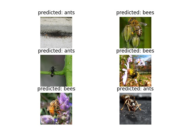
Training complete in 0m 34s
Best val Acc: 0.960784可视化模型预测结果.
visualize_model(model_conv)

plt.ioff()
plt.show()