原文：How Convolutional Layers Work in Deep Learning Neural Networks? - 2020.11.02

卷积层是深度网络中的主要构建模块，其设计灵感来源于视觉皮层(visual cortex)，其中，每个神经单元对特定视野区域(即，感受野)作出响应. 所有接受野的重叠集合可以覆盖整个视觉可见区域.

卷积层起始应用于计算机视觉，但其平移不变性(shift-invariant) 使得其可以用于自然语言处理、时间序列、推荐系统、信号处理等.

卷积层的最简单的理解是，将其看作是应用于矩阵的滑窗函数. 这里，以 1D 卷积的工作原理为例，来探索其每个参数的作用：

• kernel size
• padding
• stride
• dilation
• groups

1. Kernel size=1

卷积层是一种线性操作，其是输入和权重的乘积来得到输出.

假设 kernel (也叫权重，weights) 是 2，其原理如：

图：kernel size 为 1 的卷积操作.

对应的实现如：

class TestConv1d(nn.Module):
    def __init__(self):
        super(TestConv1d, self).__init__()
        self.conv = nn.Conv1d(in_channels=1, out_channels=1, kernel_size=1, bias=False)
        self.init_weights()

    def forward(self, x):
        return self.conv(x)
    
    def init_weights(self):
        self.conv.weight[0,0,0] = 2.

#
in_x = torch.tensor([[[1,2,3,4,5,6]]]).float()
print("in_x.shape", in_x.shape)
print(in_x)

net = TestConv1d()
out_y = net(in_x)

print("out_y.shape", out_y.shape)
print(out_y)

输出如：

in_x.shape torch.Size([1, 1, 6])
tensor([[[1., 2., 3., 4., 5., 6.]]])
out_y.shape torch.Size([1, 1, 6])
tensor([[[ 2.,  4.,  6.,  8., 10., 12.]]], grad_fn=<SqueezeBackward1>)

2. Kernel size=2

如图：

图：kernel size 为 2 的卷积操作.

其实现如：

class TestConv1d(nn.Module):
    def __init__(self):
        super(TestConv1d, self).__init__()
        self.conv = nn.Conv1d(in_channels=1, out_channels=1, kernel_size=2, bias=False)
        self.init_weights()

    def forward(self, x):
        return self.conv(x)
    
    def init_weights(self):
        self.conv.weight[0,0,0] = 2.
        self.conv.weight[0,0,1] = 2.

#
in_x = torch.tensor([[[1,2,3,4,5,6]]]).float()
print("in_x.shape", in_x.shape)
print(in_x)

net = TestConv1d()
out_y = net(in_x)

print("out_y.shape", out_y.shape)
print(out_y)

输出如：

in_x.shape torch.Size([1, 1, 6])
tensor([[[1., 2., 3., 4., 5., 6.]]])
out_y.shape torch.Size([1, 1, 5])
tensor([[[ 6., 10., 14., 18., 22.]]], grad_fn=<SqueezeBackward1>)

3. 输出向量 shape 计算

参考：torch.nn.Conv1d

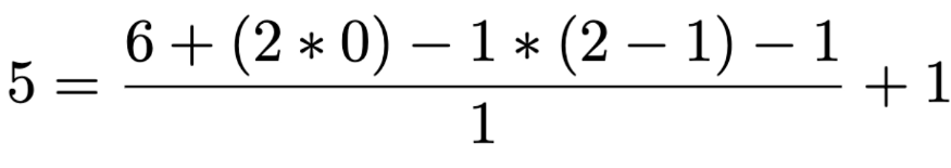
卷积输出向量长度计算：

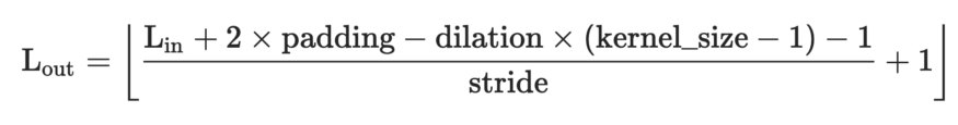
例如，采用 kernel size 为 1x2 对 1x6 输入向量进行处理，可以得到 1x5 的输出向量：

4. Kernel size=3

实际应用中， kernel size=2 是比较少见的，一般 kernel size 是奇数的. 如，kernel size=3, 如图：

图：kernel size 为 3 的卷积操作.

图像处理中，kernel size 通用的是 3x3，5x5, 或者对于较大的输入图像采用 7x7.

其实现如：

class TestConv1d(nn.Module):
    def __init__(self):
        super(TestConv1d, self).__init__()
        self.conv = nn.Conv1d(in_channels=1, out_channels=1, kernel_size=3, bias=False)
        self.init_weights()

    def forward(self, x):
        return self.conv(x)
    
    def init_weights(self):
        new_weights = torch.ones(self.conv.weight.shape) * 2.
        self.conv.weight = torch.nn.Parameter(new_weights, requires_grad=False)

#
in_x = torch.tensor([[[1,2,3,4,5,6]]]).float()
print("in_x.shape", in_x.shape)
print(in_x)

net = TestConv1d()
out_y = net(in_x)

print("out_y.shape", out_y.shape)
print(out_y)

输出如：

in_x.shape torch.Size([1, 1, 6])
tensor([[[1., 2., 3., 4., 5., 6.]]])
out_y.shape torch.Size([1, 1, 4])
tensor([[[12., 18., 24., 30.]]])

5. Padding

一般情况下，kernel 从向量的左边开始，然后对输入向量进行逐元素处理，直到最右边的最后一个元素.

kernel size 越大，则卷积的输出向量的长度越小.

如果需要输出向量的 size 和输入向量保持一致时，则需要使用 padding 操作. 其一般是在输入向量的首部和末尾处添加 0 元素.

如图：

图：kernel size 为 3 且 padding 的卷积操作.

可知，通过在输入向量的首部和末尾添加 2 个 paddings，则可保持输出向量的长度与输入向量长度一致.

对图像而言，采用 3x3 kernel 对 128x128 图像处理，可以在图像的最外圈添加 padding，以输出 128x128 的 feature map.

kernel size 为 1x3 的实现如：

class TestConv1d(nn.Module):
    def __init__(self):
        super(TestConv1d, self).__init__()
        self.conv = nn.Conv1d(in_channels=1, out_channels=1, kernel_size=3, padding=1, bias=False)
        self.init_weights()

    def forward(self, x):
        return self.conv(x)
    
    def init_weights(self):
        new_weights = torch.ones(self.conv.weight.shape) * 2.
        self.conv.weight = torch.nn.Parameter(new_weights, requires_grad=False)

#
in_x = torch.tensor([[[1,2,3,4,5,6]]]).float()
print("in_x.shape", in_x.shape)
print(in_x)

net = TestConv1d()
out_y = net(in_x)

print("out_y.shape", out_y.shape)
print(out_y)

输出如：

in_x.shape torch.Size([1, 1, 6])
tensor([[[1., 2., 3., 4., 5., 6.]]])
out_y.shape torch.Size([1, 1, 6])
tensor([[[ 6., 12., 18., 24., 30., 22.]]])

kernel size 为 1x5 的实现如：

class TestConv1d(nn.Module):
    def __init__(self):
        super(TestConv1d, self).__init__()
        self.conv = nn.Conv1d(in_channels=1, out_channels=1, kernel_size=5, padding=2, bias=False)
        self.init_weights()

    def forward(self, x):
        return self.conv(x)
    
    def init_weights(self):
        new_weights = torch.ones(self.conv.weight.shape) * 2.
        self.conv.weight = torch.nn.Parameter(new_weights, requires_grad=False)

#
in_x = torch.tensor([[[1,2,3,4,5,6]]]).float()
print("in_x.shape", in_x.shape)
print(in_x)

net = TestConv1d()
out_y = net(in_x)

print("out_y.shape", out_y.shape)
print(out_y)

输出如：

in_x.shape torch.Size([1, 1, 6])
tensor([[[1., 2., 3., 4., 5., 6.]]])
out_y.shape torch.Size([1, 1, 6])
tensor([[[12., 20., 30., 40., 36., 30.]]])

6. Stride

上面都是以步长为 1 进行滑窗，通过增加步长大小(stride size) 可以平移特定数量的元素. 如图：

图：kernel size 为 3，stride=3 的卷积操作.

大部分情况下，增加步长是为了对输入向量进行下采样. stride=2 则输出向量长度减半. 在某些情况下，采用大步长来取代 pooling 层，来降低 spatial 大小、降低模型参数、增加速度等.

其实现如：

class TestConv1d(nn.Module):
    def __init__(self):
        super(TestConv1d, self).__init__()
        self.conv = nn.Conv1d(in_channels=1, out_channels=1, kernel_size=3, stride=3, bias=False)
        self.init_weights()

    def forward(self, x):
        return self.conv(x)
    
    def init_weights(self):
        new_weights = torch.ones(self.conv.weight.shape) * 2.
        self.conv.weight = torch.nn.Parameter(new_weights, requires_grad=False)

#
in_x = torch.tensor([[[1,2,3,4,5,6]]]).float()
print("in_x.shape", in_x.shape)
print(in_x)

net = TestConv1d()
out_y = net(in_x)

print("out_y.shape", out_y.shape)
print(out_y)

输出如：

in_x.shape torch.Size([1, 1, 6])
tensor([[[1., 2., 3., 4., 5., 6.]]])
out_y.shape torch.Size([1, 1, 2])
tensor([[[12., 30.]]])

7. Dilation

深度网络中， Dilated convolutions 通过在 kernel 元素见插入空格来膨胀(inflate) kernel，并由一个参数来控制 dilation rate.

dilation rate=2 表示 kernel 元素间有一个空格(space).

dilation rate=1 则等价于正常卷积.

dialtion convs 能够有效增加输出向量的接受野，且不增加 kernel size 与模型大小.

参考：DeepLab: Semantic Image Segmentation with Deep Convolutional Nets, Atrous Convolution, and Fully Connected CRFs - 2016

如图：

图：kernel size 为 3，dilation rate=2 的卷积操作.

通常情况下，dilated convs 对于图像分割任务能够有较好的表现. 如果想在不损失分辨率的情况下，对接受野进行指数扩展，也可以使用 dilated convs.

其实现如：

class TestConv1d(nn.Module):
    def __init__(self):
        super(TestConv1d, self).__init__()
        self.conv = nn.Conv1d(in_channels=1, out_channels=1, kernel_size=3, dilation=2, bias=False)
        self.init_weights()

    def forward(self, x):
        return self.conv(x)
    
    def init_weights(self):
        new_weights = torch.ones(self.conv.weight.shape) * 2.
        self.conv.weight = torch.nn.Parameter(new_weights, requires_grad=False)

#
in_x = torch.tensor([[[1,2,3,4,5,6]]]).float()
print("in_x.shape", in_x.shape)
print(in_x)

net = TestConv1d()
out_y = net(in_x)

print("out_y.shape", out_y.shape)
print(out_y)

输出如：

in_x.shape torch.Size([1, 1, 6])
tensor([[[1., 2., 3., 4., 5., 6.]]])
out_y.shape torch.Size([1, 1, 2])
tensor([[[18., 24.]]])

8. Groups

卷积默认 groups=1，表示所有的输入通道都被卷积到所有输出.

groupwise convolution 则需要增加 groups 值，其将强制把输入向量通道(channels) 划分为不同的特征组(groupings of features).

groups=2,其等价于并排两个卷积层，每个仅处理一半的输入通道. 然后，每个 group 输出一半的输出通道，最后合并链接得到最终的输出向量.

如图：

图：groupwise convolution

其实现如：

class TestConv1d(nn.Module):
    def __init__(self):
        super(TestConv1d, self).__init__()
        self.conv = nn.Conv1d(in_channels=2, out_channels=2, kernel_size=1, groups=2, bias=False)
        self.init_weights()

    def forward(self, x):
        return self.conv(x)
    
    def init_weights(self):
        print(self.conv.weight.shape)
        self.conv.weight[0,0,0] = 2.
        self.conv.weight[1,0,0] = 4.

#
in_x = torch.tensor([[[1,2,3,4,5,6],[10,20,30,40,50,60]]]).float()
print("in_x.shape", in_x.shape)
print(in_x)

net = TestConv1d()
out_y = net(in_x)

print("out_y.shape", out_y.shape)
print(out_y)

输入如：

in_x.shape torch.Size([1, 2, 6])
tensor([[[ 1.,  2.,  3.,  4.,  5.,  6.],
         [10., 20., 30., 40., 50., 60.]]])
torch.Size([2, 1, 1])
out_y.shape torch.Size([1, 2, 6])
tensor([[[  2.,   4.,   6.,   8.,  10.,  12.],
         [ 40.,  80., 120., 160., 200., 240.]]], grad_fn=<SqueezeBackward1>)

Groups 参数被用于 Depthwise convolution 的实现，如，需要对 R, G, B 通道分别提取图像特征时.

当 groups==in_channels，out_channles=Kxin_channels 时，这种操作也被在 depthwise convolution 中提及.

其实现如：

class TestConv1d(nn.Module):
    def __init__(self):
        super(TestConv1d, self).__init__()
        self.conv = nn.Conv1d(in_channels=2, out_channels=4, kernel_size=1, groups=2, bias=False)
        self.init_weights()

    def forward(self, x):
        return self.conv(x)
    
    def init_weights(self):
        print(self.conv.weight.shape)
        self.conv.weight[0,0,0] = 2.
        self.conv.weight[1,0,0] = 4.
        self.conv.weight[2,0,0] = 6.
        self.conv.weight[3,0,0] = 8.

#
in_x = torch.tensor([[[1,2,3,4,5,6],[10,20,30,40,50,60]]]).float()
print("in_x.shape", in_x.shape)
print(in_x)

net = TestConv1d()
out_y = net(in_x)

print("out_y.shape", out_y.shape)
print(out_y)

输出如：

in_x.shape torch.Size([1, 2, 6])
tensor([[[ 1.,  2.,  3.,  4.,  5.,  6.],
         [10., 20., 30., 40., 50., 60.]]])
torch.Size([4, 1, 1])
out_y.shape torch.Size([1, 4, 6])
tensor([[[  2.,   4.,   6.,   8.,  10.,  12.],
         [  4.,   8.,  12.,  16.,  20.,  24.],
         [ 60., 120., 180., 240., 300., 360.],
         [ 80., 160., 240., 320., 400., 480.]]], grad_fn=<SqueezeBackward1>)

在 2012 年 AlexNet 论文里，grouped convolution 被提出，其主要动机是为了将网络能够在两张 GPUs 上进行训练.

9. 1x1 conv

Network in Network 首先使用了 1x1 conv，其容易迷惑的地方在于，其作用好像只是逐点乘积. 但其作用实际上不仅仅如此. 如，在计算机视觉中，如果输入是 128x128x3, 由于其 depth 通道为 3, 则1x1 conv 能够有效的进行 3-dim 点积计算.

GoogLeNet 中 1x1 conv 被用于降维和增加 feature maps 的维度.

ResNet 中 1x1 conv 被用于在残差网络中，投影(projection technique) 以匹配输入的 filiters 数和残差输出模块.

TCN 中因为输入和输出 widths 可能不同，所以 1x1 kernel 被添加，以解决输入输出 widths 的差异. 1x1 conv 可确保逐元素加法，接收相同 shape 的张量.

一文读懂卷积神经网络中的1x1卷积核 - 2018.07.19

卷积神经网络中用1*1 卷积有什么作用或者好处呢？- 知乎