题目: Focal Loss for Dense Object Detection - ICCV2017

作者: Tsung-Yi, Lin, Priya Goyal, Ross Girshick, Kaiming He, Piotr Dollar

团队: FAIR

<Detectron>

精度最高的目标检测器往往基于 RCNN 的 two-stage 方法，对候选目标位置再采用分类器处理. 而，one-stage 目标检测器是对所有可能的目标位置进行规则的(regular)、密集采样，更快速简单，但是精度还在追赶 two-stage 检测器. <论文所关注的问题于此.>

论文发现，密集检测器训练过程中，所遇到的极端前景背景类别不均衡(extreme foreground-background class imbalance) 是核心原因.

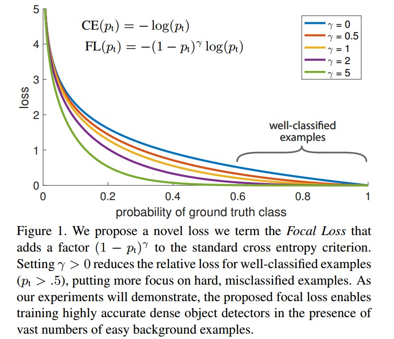
对此，提出了 Focal Loss，通过修改标准的交叉熵损失函数，降低对能够很好分类样本的权重(down-weights the loss assigned to well-classified examples)，解决类别不均衡问题.

Focal Loss 关注于在 hard samples 的稀疏子集进行训练，并避免在训练过程中大量的简单负样本淹没检测器. <RetinaNet>

Focal Loss 是动态缩放的交叉熵损失函数，随着对正确分类的置信增加，缩放因子(scaling factor) 衰退到 0. 如图：

Focal Loss 的缩放因子能够动态的调整训练过程中简单样本的权重，并让模型快速关注于困难样本(hard samples).

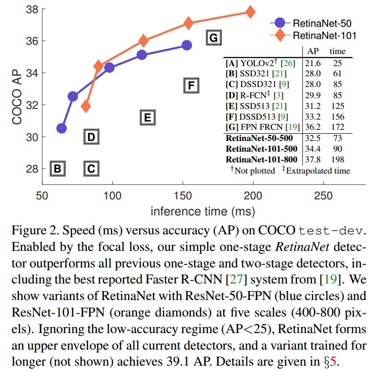
基于 Focal Loss 的 RetinaNet 的目标检测器表现.

1. Focal Loss

Focal Loss 旨在解决 one-stage 目标检测器在训练过程中出现的极端前景背景类不均衡的问题(如，前景：背景 = 1:1000).

首先基于二值分类的交叉熵(cross entropy, CE) 引入 Focal Loss：

$$ CE(p, y) = \begin{cases} -log(p) &\text{if } y=1 \\ -log(1-p) &\text{otherwise } \end{cases} $$

其中，$y \in \lbrace +1 -1 \rbrace$ 为 groundtruth 类别；$p \in [0, 1]$ 是模型对于类别 $y=1$ 所得到的预测概率.

符号简介起见，定义 $p_t$：

$$ p_t = \begin{cases} p &\text{if } y=1 \\ 1-p &\text{otherwise } \end{cases} $$

则，$CE(p, y) = CE(p_t) = -log(p_t)$.

CE Loss 如图 Figure 1 中的上面的蓝色曲线所示. 其一个显著特点是，对于简单易分的样本，如，$p_t \gg 0.5$，其 loss 也是一致对待. 当累加了大量简单样本的 loss 后，具有很小 loss 值的可能淹没稀少的类(rare class).

1.1 均衡交叉熵 Blanced CE

解决类别不均衡的一种常用方法是，对类别 +1 引入权重因子 $\alpha \in [0, 1]$，对于类别 -1 引入权重 $1 - \alpha$.

符号简介起见，定义 $\alpha _t$：

$$ \alpha_t = \begin{cases} \alpha &\text{if } y=1 \\ 1-\alpha &\text{otherwise } \end{cases} $$

则，$\alpha$-balanced CE loss 为：

$$ CE(p_t) = -\alpha _t log(p_t) $$

1.2 Focal Loss 定义

虽然 $\alpha$ 能够平衡 positive/negative 样本的重要性，但不能区分 easy/hard 样本.

对此，Focal Loss 提出将损失函数降低 easy 样本的权重，并关注于对 hard negatives 样本的训练.

添加调制因子(modulating factor) $(1 - p_t)^{\gamma}$ 到 CE loss，其中 $\gamma \ge 0$ 为可调的 focusing 参数.

Focal Loss 定义为：

$$ FL(p_t) = -(1 - p_t)^{\gamma} log(p_t) $$

如图 Figure 1，给出了 $\gamma \in [0, 5]$ 中几个值的可视化.

Focal Loss 的两个属性：

[1] - 当样本被误分，且 $p_t$ 值很小时，调制因子接近于 1，loss 不受影响. 随着 $p_t \rightarrow 1$，则调制因子接近于 0，则容易分类的样本的损失函数被降低权重.

[2] - focusing 参数 $\gamma$ 平滑地调整哪些 easy 样本会被降低权重的比率(rate). 当 $\gamma=0$，FL=CE；随着 $\gamma $ 增加，调制因子的影响也会随之增加(实验中发现 $\gamma = 2$ 效果最佳.)

直观上，调制因子能够减少 easy 样本对于损失函数的贡献，并延伸了loss 值比较地的样本范围.

例如，$\gamma = 0.2$ 时，被分类为 $p_t=0.9$ 的样本，与 CE 相比，会减少 100x 倍；而且，被分类为 $p_t \approx 0.968 $ 的样本，与 CE 相比，会有少于 1000x 倍的 loss 值. 这就自然增加了将难分类样本的重要性(如 $\gamma= 2$ 且 $p_t \leq 0.5$ 时，难分类样本的 loss 值会增加 4x 倍.)

实际上，论文采用了 Focal Loss 的 $\alpha$ -balanced 变形：

$$ FL(p_t) = -\alpha _t (1 - p_t)^{\gamma} log(p_t) $$

1.3. Focal Loss 例示

Focal Loss 并不局限于具体的形式. 这里给出另一种例示.

假设 $p = \sigma(x) = \frac{1}{1 + e^{-x}}$，

定义 $p_t$为(类似于前面对于 $p_t$ 的定义)：

$$ p_t = \begin{cases} p &\text{if } y=1 \\ 1-p &\text{otherwise } \end{cases} $$

定义：$x_t = yx$，其中，$y \in \lbrace +1, -1 \rbrace$ 是 groundtruth 类别.

则：

$$ p_t = \sigma(x_t) = \frac{1}{1 + e^{-yx}} $$

当 $x_t > 0$ 时，样本被正确分类，此时 $p_t > 0.5$.

有：

$$ \frac{d p_t}{d x} = \frac{-1}{(1 + e^{-yx})^2} * (-y) * e^{-yx} = y * p_t * (1 - p_t) = -y * p_t * (p_t - 1) $$

对于交叉熵损失函数 $CE(p_t) = -log(p_t)$，由$\frac{d lnx}{d x} = \frac{1}{x}$，

$$ \frac{d CE(p_t)}{d x} = \frac{d CE(p_t)}{d p_t} * \frac{d p_t}{d x} = (- \frac{1}{p_t}) * (-y*p_t*(p_t - 1)) = y*(p_t - 1) $$

对于 Focal Loss $FL(p_t) = -(1 - p_t)^{\gamma} log(p_t)$，其中 $\gamma$ 为常数.

$$ \frac{d FL(p_t)}{d x} = \frac{d (1-p_t)^{\gamma}}{d x} * (-log(p_t)) + (1-p_t)^{\gamma}*\frac{d CE(p_t)}{d x} $$

$$ \frac{d FL(p_t)}{d x} = (\gamma * (1-p_t)^{\gamma-1}*\frac{d (1-p_t)}{d p_t})*\frac{d p_t}{d x} * (-log(p_t)) + (1-p_t)^{\gamma}*y*(p_t -1) $$

$$ \frac{d FL(p_t)}{d x} = (\gamma *(1- p_t)^{\gamma -1} * (-1))*(-y * p_t*(p_t -1))*(-log(p_t)) + y*(1-p_t)^{\gamma}*(p_t -1) $$

$$ \frac{d FL(p_t)}{d x} = \gamma *(1-p_t)^{\gamma}*y*p_t*log(p_t) + y*(1-p_t)^{\gamma}*(p_t - 1) $$

$$ \frac{d FL(p_t)}{d x} = y*(1-p_t)^{\gamma}*(\gamma * p_t *log(p_t) + (p_t - 1)) $$

再者，假设 $p_t^* = \sigma (\gamma x_t + \beta)$，则 $FL^*(p_t^{*}) = -log(p_t^*)/ \gamma$，其中 $\gamma$ 为常数.

$$ \frac{d FL^*(p_t^*)}{d x} = -\frac{1}{p_t^*}*\frac{1}{\gamma}*\frac{d p_t^*}{d (\gamma x_t + \beta)} * \frac{d( \gamma x_t + \beta)}{d x} $$

$$ \frac{d FL^*(p_t^*)}{d x} = -\frac{1}{p_t^*} * \frac{1}{\gamma} * (-y * p_t^* * (p_t^* - 1)*\gamma) = y*(p_t^* - 1) $$

则，$FL^*$ 包含两个参数 $\gamma$ 和 $\beta$，控制着 loss 曲线的陡度(steepness) 和移动(shift). 如 Figure 5.

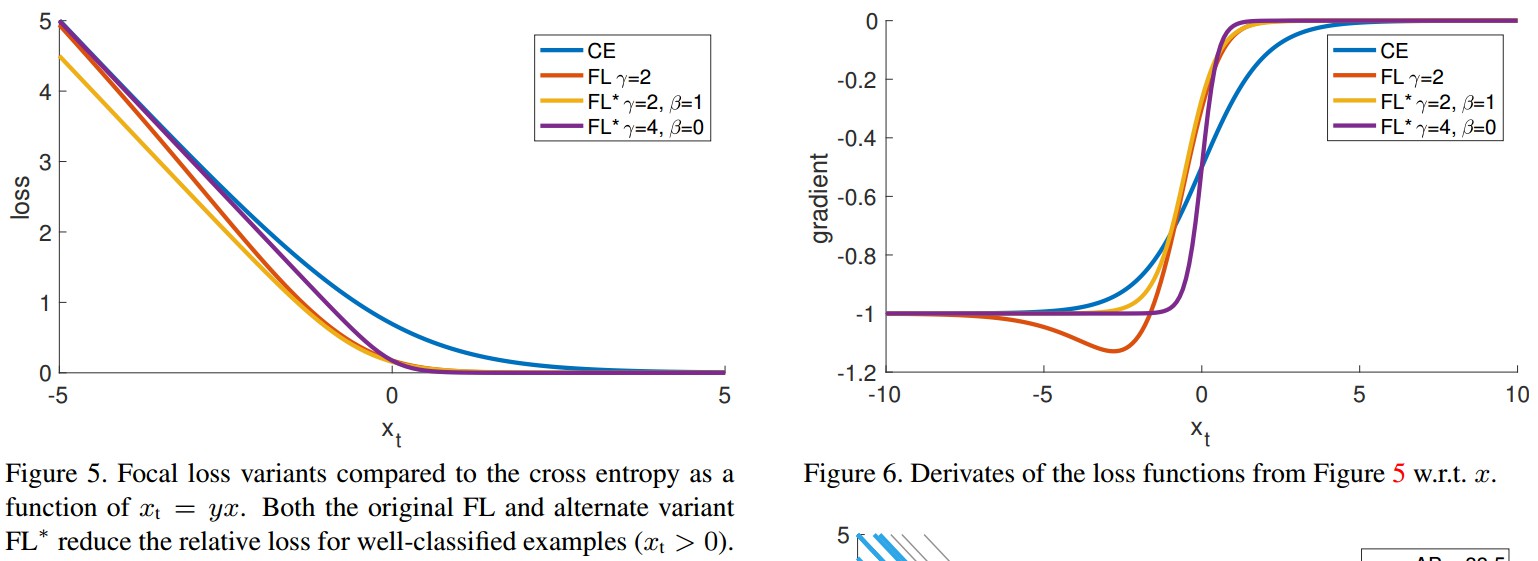
1.4. Focal Loss 求导

$CE$ 关于 $x$ 的求导：

$$ \frac{d CE}{ dx} = y(p_t - 1) $$

$FL$ 关于 $x$ 的求导：

$$ \frac{d FL}{d x} = y(1-p_t)^{\gamma} (\gamma p_t log(p_t) + p_t - 1) $$

$FL^*$ 关于 $x$ 的求导：

$$ \frac{d FL^*}{d x} = y(p_t^* - 1) $$

如图 Figure 6. 三种 loss 函数，对于high-confidence 的预测结果，其导数都趋近于 -1 或 0.

但，与 $CE$ 不同的是，$FL$ 和 $FL^*$ 的有效设置时，只要 $x_t > 0$，二者的导数都是很小的.

2. SoftmaxFocalLoss 求导

Focal Loss 损失函数：

$$ FL(p_t) = - \alpha (1 - p_t)^{\gamma} log(p_t) $$

其中：

$$ p_t = \begin{cases} p &\text{if } y=1 \\ 1-p &\text{otherwise } \end{cases} $$

Softmax 函数：

$$ p_i = \frac{e^{x_i}}{\sum _{k=1}^K e^{x_k}} $$

其中，$K$ 为类别数，$x$ 是网络全连接层等的输出向量，$x_i$ 是向量的第 $i$ 个元素值.

则 $FL$ 关于 $x$ 求导：

$$ \frac{d FL}{d x_i} = \frac{d FL}{d p_i} * \frac{d p_i}{d x_i} $$

而，

$$ \frac{d FL}{d p_t} = - \alpha (\frac{d (1-p_t)^{\gamma}}{d p_t} * log(p_t) + (1-p_t)^{\gamma} * \frac{d (log(p_t))}{d p_t}) $$

$$ \frac{d FL}{d p_t} = - \alpha (- \gamma * (1-p_t)^{\gamma - 1} * log(p_t) + (1-p_t)^{\gamma} * \frac{1}{p_t}) $$

Softmax 函数关于 x 的求导为：

$$ \frac{d p_i}{d x_i} = \frac{d \frac{e^{x_i}}{\sum _{k=1}^K e^{x_k}}}{d x_i} $$

$$ \frac{d p_i}{d x_i} = \frac{\frac{d(e^{x_i})}{d x_i}*\sum _{k=1}^K e^{x_k} - e^{x_i}*\frac{d(\sum _{k=1}^K e^{x_k})}{dx_i}}{(\sum _{k=1}^K e^{x_k})^2} $$

当 $i=j$ 时，

$$ \frac{d p_i}{d x_i} = \frac{e^{x_i}*\sum _{k=1}^K e^{x_k} - e^{x_i}*e^{x_i}}{(\sum _{k=1}^K e^{x_k})^2} $$

$$ \frac{d p_i}{d x_i} = \frac{e^{x_i}}{\sum _{k=1}^K e^{x_k}} - \frac{e^{x_i}}{\sum _{k=1}^K e^{x_k}}* \frac{e^{x_i}}{\sum _{k=1}^K e^{x_k}} $$

$$ \frac{d p_i}{d x_i} = p_i - p_i * p_i = p_i(1 - p_i) $$

当 $i \neq j$ 时，

$$ \frac{d p_i}{d x_i} = \frac{0 - e^{x_i}*e^{x_j}}{(\sum _{k=1}^K e^{x_k})^2} $$

$$ \frac{d p_i}{d x_i} = - \frac{e^{x_i}}{\sum _{k=1}^K e^{x_k}}* \frac{e^{x_j}}{\sum _{k=1}^K e^{x_k}} $$

$$ \frac{d p_i}{d x_i} = -p_i * p_j $$

Softmax 的函数求导即为：

$$ \frac{d p_i}{d x_i} = \begin{cases} p_i(1-p_i) &\text{if } i=j \\ -p_i*p_j &\text{if } i \neq j \end{cases} $$

故：

$$ \frac{d FL}{d x_i} = \begin{cases} - \alpha (- \gamma * (1-p_i)^{\gamma - 1} * log(p_i) + (1-p_i)^{\gamma} * \frac{1}{p_i}) * p_i(1-p_i) &\text{if } i=j \\ - \alpha (- \gamma * (1-p_i)^{\gamma - 1} * log(p_i) + (1-p_i)^{\gamma} * \frac{1}{p_i}) * (-p_i*p_j) &\text{if } i \neq j \end{cases} $$

$$ \frac{d FL}{d x_i} = \begin{cases} \alpha (- \gamma * (1-p_i)^{\gamma - 1} * log(p_i)p_i + (1-p_i)^{\gamma}) * (p_i-1) &\text{if } i=j \\ \alpha (- \gamma * (1-p_i)^{\gamma - 1} * log(p_i)p_i + (1-p_i)^{\gamma}) * p_j &\text{if } i \neq j \end{cases} $$

3. Pytorch 实现

FocalLoss-PyTorch

import torch
import torch.nn as nn
import torch.nn.functional as F

class FocalLoss(nn.Module):
    def __init__(self, alpha=0.25, gamma=2, size_average=True):
        super(FocalLoss, self).__init__()
        self.alpha = alpha
        self.gamma = torch.Tensor([gamma])
        self.size_average = size_average
        if isinstance(alpha, (float, int, long)):
            if self.alpha > 1:
                raise ValueError('Not supported value, alpha should be small than 1.0')
            else:
                self.alpha = torch.Tensor([alpha, 1.0 - alpha])
        if isinstance(alpha, list): self.alpha = torch.Tensor(alpha)
        self.alpha /= torch.sum(self.alpha)

    def forward(self, input, target):
        if input.dim() > 2:
            input = input.view(input.size(0), input.size(1), -1)  # [N,C,H,W]->[N,C,H*W] ([N,C,D,H,W]->[N,C,D*H*W])
        # target
        # [N,1,D,H,W] ->[N*D*H*W,1]
        if self.alpha.device != input.device:
            self.alpha = torch.tensor(self.alpha, device=input.device)
        target = target.view(-1, 1)
        logpt = torch.log(input + 1e-10)
        logpt = logpt.gather(1, target)
        logpt = logpt.view(-1, 1)
        pt = torch.exp(logpt)
        alpha = self.alpha.gather(0, target.view(-1))

        gamma = self.gamma

        if not self.gamma.device == input.device:
            gamma = torch.tensor(self.gamma, device=input.device)

        loss = -1 * alpha * torch.pow((1 - pt), gamma) * logpt
        if self.size_average:
            loss = loss.mean()
        else:
            loss = loss.sum()
        return loss

4. Keras 实现

keras-focal-loss

基于 Keras 和 TensorFlow 后端实现的 Binary Focal Loss 和 Categorical/Multiclass Focal Loss.

主要设计两个参数：alpha 和 gamma.

用法：

model.compile(optimizer='adam', loss=categorical_focal_loss(gamma=2.0, alpha=0.25), metrics=['accuracy'])

实现：

#!/usr/bin/env python3
# -*- coding: utf-8 -*-
"""
Created on Fri Oct 19 08:20:58 2018

@OS: Ubuntu 18.04
@IDE: Spyder3
@author: Aldi Faizal Dimara (Steam ID: phenomos)
"""

import keras.backend as K
import tensorflow as tf

def categorical_focal_loss(gamma=2.0, alpha=0.25):
    """
    Implementation of Focal Loss from the paper in multiclass classification
    Formula:
        loss = -alpha*((1-p)^gamma)*log(p)
    Parameters:
        alpha -- the same as wighting factor in balanced cross entropy
        gamma -- focusing parameter for modulating factor (1-p)
    Default value:
        gamma -- 2.0 as mentioned in the paper
        alpha -- 0.25 as mentioned in the paper
    """
    def focal_loss(y_true, y_pred):
        # Define epsilon so that the backpropagation will not result in NaN
        # for 0 divisor case
        epsilon = K.epsilon()
        # Add the epsilon to prediction value
        #y_pred = y_pred + epsilon
        # Clip the prediction value
        y_pred = K.clip(y_pred, epsilon, 1.0-epsilon)
        # Calculate cross entropy
        cross_entropy = -y_true*K.log(y_pred)
        # Calculate weight that consists of  modulating factor and weighting factor
        weight = alpha * y_true * K.pow((1-y_pred), gamma)
        # Calculate focal loss
        loss = weight * cross_entropy
        # Sum the losses in mini_batch
        loss = K.sum(loss, axis=1)
        return loss
    
    return focal_loss

def binary_focal_loss(gamma=2.0, alpha=0.25):
    """
    Implementation of Focal Loss from the paper in multiclass classification
    Formula:
        loss = -alpha_t*((1-p_t)^gamma)*log(p_t)
        
        p_t = y_pred, if y_true = 1
        p_t = 1-y_pred, otherwise
        
        alpha_t = alpha, if y_true=1
        alpha_t = 1-alpha, otherwise
        
        cross_entropy = -log(p_t)
    Parameters:
        alpha -- the same as wighting factor in balanced cross entropy
        gamma -- focusing parameter for modulating factor (1-p)
    Default value:
        gamma -- 2.0 as mentioned in the paper
        alpha -- 0.25 as mentioned in the paper
    """
    def focal_loss(y_true, y_pred):
        # Define epsilon so that the backpropagation will not result in NaN
        # for 0 divisor case
        epsilon = K.epsilon()
        # Add the epsilon to prediction value
        #y_pred = y_pred + epsilon
        # Clip the prediciton value
        y_pred = K.clip(y_pred, epsilon, 1.0-epsilon)
        # Calculate p_t
        p_t = tf.where(K.equal(y_true, 1), y_pred, 1-y_pred)
        # Calculate alpha_t
        alpha_factor = K.ones_like(y_true)*alpha
        alpha_t = tf.where(K.equal(y_true, 1), alpha_factor, 1-alpha_factor)
        # Calculate cross entropy
        cross_entropy = -K.log(p_t)
        weight = alpha_t * K.pow((1-p_t), gamma)
        # Calculate focal loss
        loss = weight * cross_entropy
        # Sum the losses in mini_batch
        loss = K.sum(loss, axis=1)
        return loss
    
    return focal_loss    

Related

[1] - Focal Loss 的前向与后向公式推导