原文:End-to-End Multi-label Classification - 2020.05.08
Kaggle:Example of multi-label multi-class classification
作者:Bhartendu
1. Multi-Label classification
在机器学习领域,多标签分类及其强相关的多输出分类(multi-output classification)是分类问题的一种变形,其针对的是每个实例可以被指定多个类别标签.
多标签分类是多类别分类(multiclass classification) 的一种泛化,后者是将实例精确地分类到多个类别(超过两个)中的某个标签的单标签问题. 而,对于多标签分类问题,没有限定实例能被指定的类别标签数量.
正式地,多标签分类针对的问题是,构建输入 $\mathbf{x}$ 到二值向量 $\mathbf{y}$ 的模型,其中,向量 $\mathbf{y}$ 中的每个元素(标签)的值为 0 或 1.
这里举例说明多标签问题:
服装主体包含多个属性(标签),如颜色、图案、类目、场景等. 每个属性有其自己的类别,比如,场景可以被分类为运动(Sports)、正式(Formal)、民族(Ethnic)、休闲(Casual).
可以采用的数据集有:DeepFashion, FashionGen. 这里以 Kaggle fashion_small 数据集为例.
2. Fashion_small 数据探索
fashion_small 数据集共包含 21K 服装主体. 这里对每个标签中的每个类设置最小样本数 $\mathbf{s}$. 对于每个标签中的所有类设置固定的数量.
最小样本数:$\mathcal{s} = 700$.
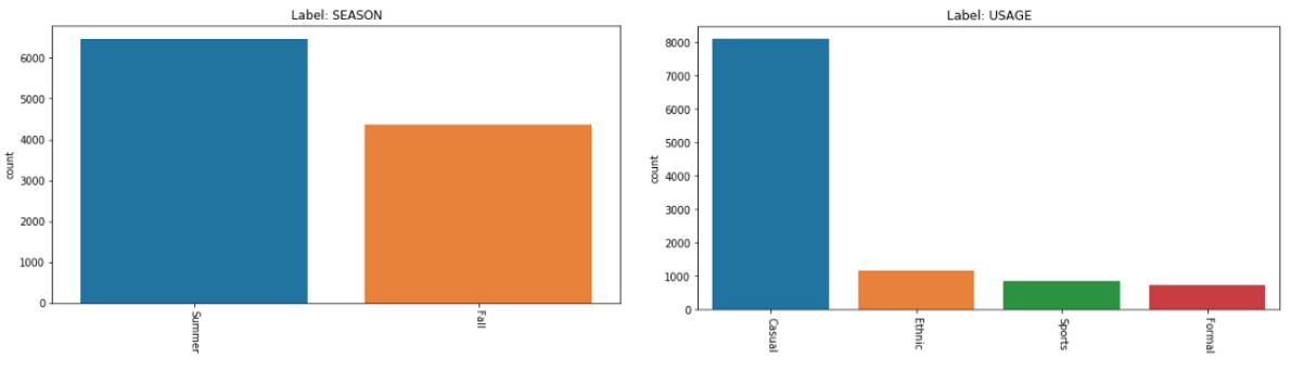
如图,为每个标签的条形图(移除数量小于 $\mathcal{s}$ 的类):
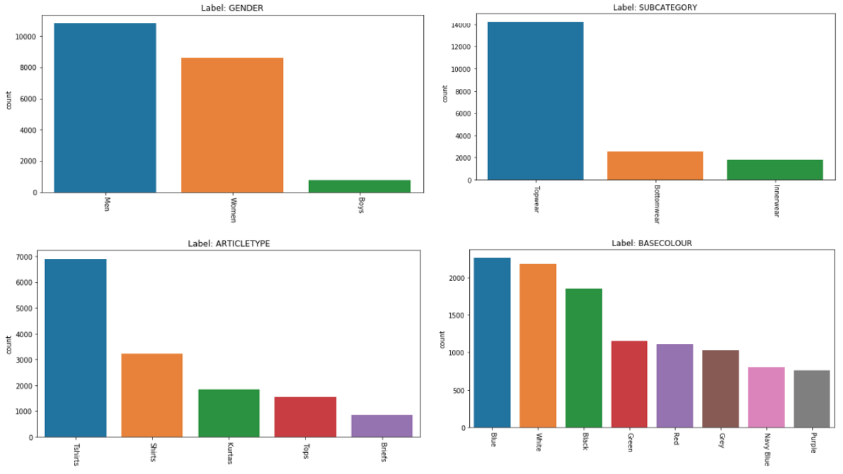
Attributes | Number of classes
-------------------------------------------------
gender | 3
subCategory | 2
articleType | 5
baseColour | 8
season | 2
usage | 4
--------------------------------------------------
Total number of label | 6
Total number of classes | 24
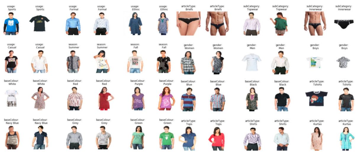
Total number of images | 10809样例图片如下(不同标签的不同类):
最终的数据组织形式为(DataFrame):
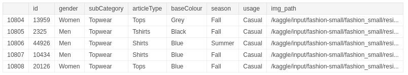
因此,最终服装主体识别问题为,多标签(6个)多类别(24个)问题.
2.1. 数据探索完整实现
该部分的代码实现为:
import os
import json
import warnings
warnings.filterwarnings('ignore')

import pandas as pd
import numpy as np
import seaborn as sns

import matplotlib.image as mpimg
import matplotlib.pyplot as plt

from collections import Counter, defaultdict
from sklearn.model_selection import train_test_split
from sklearn.preprocessing import LabelEncoder

from keras.preprocessing import image
from keras.models import Model, load_model
from keras.layers import Input, Dense, Dropout, Conv2D, MaxPooling2D
from keras.layers import BatchNormalization, add, GlobalAveragePooling2D
from keras.callbacks import EarlyStopping, ModelCheckpoint
from keras.utils.np_utils import to_categorical
from keras.utils import plot_model

#
path = '/path/to/fashion_small/'
table = 'styles.csv'
base = path+'resized_images/'
print('\nDirectory contains:\n', os.listdir(path))

data = pd.read_csv(path+table, error_bad_lines=False, warn_bad_lines=False)
print('\n CSV contains {} entries, with attributes\n {}'.format(len(data),data.keys().values))
'''
 CSV contains 44424 entries, with attributes
 ['id' 'gender' 'masterCategory' 'subCategory' 'articleType' 'baseColour'
 'season' 'year' 'usage' 'productDisplayName']
'''

# Check for exsisting images in database
im_path = []
for item_id in data['id']:
    tmp_path = base + str(item_id) +'.jpg'
    if os.path.exists(tmp_path):
        im_path.append(tmp_path)
    else:
        data.drop(data[data.id == item_id].index, inplace=True)
        print('Item {} Doesn\'t exists'.format(item_id))

data['img_path'] = im_path
data = data.sample(frac=1, random_state=10)
data.dropna(inplace=True)
data.reset_index(drop=True, inplace=True)
data.tail()
'''
Item 39403 Doesn't exists
Item 39410 Doesn't exists
Item 39401 Doesn't exists
Item 39425 Doesn't exists
Item 12347 Doesn't exists
'''

#Unique values per column
data.nunique()
'''
id                    44072
gender                    5
masterCategory            7
subCategory              45
articleType             141
baseColour               46
season                    4
year                     13
usage                     8
productDisplayName    30801
img_path              44072
dtype: int64
'''

# Analysing Apparels from masterCategory
# a. Removing Duplicate entries
# b. Removing 'year' :: Can't be learnt visually
# c. Removing 'productDisplayName' :: Can't be learnt visually
df = data[data['masterCategory'] == 'Apparel']
df.drop_duplicates(subset='img_path', inplace=True)
df.drop(columns=['masterCategory', 'year', 'productDisplayName'], inplace=True)
df.reset_index(inplace=True, drop=True)
df.tail(5)
辅助函数:
# Temp functions
# a. Display Categorical charts
# b. Clean dataFrame as per minimum requirements for modelling
def disp_category(category, df, min_items=500):
    '''
    Display Categorical charts
    category  :: dtpye=str, Category (attribute/column name)
    df        :: DataFrame to be loaded
    min_items :: dtype=int, minimum rows to qualify as class

    returns classes to be selected for the analysis
    '''
    dff = df.groupby(category)
    class_ = dff.count().sort_values(by='id')['id'].reset_index()
    class_.columns=[category,'count']

    class_= class_[class_['count']>=min_items][category]
    df = df[df[category].isin(class_)]

    labels = df[category]
    counts = defaultdict(int)
    for l in labels:
         counts[l] += 1

    counts_df = pd.DataFrame.from_dict(counts, orient='index')
    counts_df.columns = ['count']
    counts_df.sort_values('count', ascending=False, inplace=True)

    #
    fig, ax = plt.subplots()
    ax = sns.barplot(x=counts_df.index, y=counts_df['count'], ax=ax)
    fig.set_size_inches(10,5)
    ax.set_xticklabels(ax.xaxis.get_majorticklabels(), rotation=-90);
    ax.set_title('Label: '+category.upper())
    plt.show()
    return class_


def reduce_df(df, category, class_):
    '''
    Remove noise points from dataFrame
    category  :: dtpye=str, Category (attribute/column name)
    df        :: DataFrame to be loaded
    class_    :: list, classes to be seleted for the analysis

    returns: clean dataFrame
    '''
    print('Analysing {} as feature'.format(category))
    print('Prior Number of datapoints: {}  ::  Classes: {}'.format(
        len(df), set(df[category])))
    df = df[df[category].isin(class_)]
    df.reset_index(drop=True, inplace=True)
    print('Posterior Number of datapoints: {}  ::  Classes: {}\n'.format(
        len(df), set(df[category])))
    return df
标签分析:
# Analysing labels
# Minmum requirement: set minimum samples per class
for cate in df.keys()[1:-1]:
    class_ = disp_category(cate, df, min_items=700)
    df = reduce_df(df, cate, class_)
'''
Analysing gender as feature
Prior Number of datapoints: 21361  ::  Classes: {'Boys', 'Girls', 'Unisex', 'Men', 'Women'}
Posterior Number of datapoints: 20709  ::  Classes: {'Boys', 'Men', 'Women'}

Analysing subCategory as feature
Prior Number of datapoints: 20709  ::  Classes: {'Topwear', 'Loungewear and Nightwear', 'Bottomwear', 'Socks', 'Apparel Set', 'Saree', 'Innerwear', 'Dress'}
Posterior Number of datapoints: 19307  ::  Classes: {'Topwear', 'Bottomwear', 'Innerwear'}

Analysing articleType as feature
Prior Number of datapoints: 19307  ::  Classes: {'Sweaters', 'Tights', 'Boxers', 'Churidar', 'Jeggings', 'Suspenders', 'Salwar', 'Swimwear', 'Rompers', 'Belts', 'Nehru Jackets', 'Shirts', 'Tracksuits', 'Skirts', 'Shapewear', 'Lehenga Choli', 'Waistcoat', 'Tunics', 'Sweatshirts', 'Track Pants', 'Briefs', 'Jeans', 'Salwar and Dupatta', 'Trunk', 'Bra', 'Rain Jacket', 'Dresses', 'Innerwear Vests', 'Trousers', 'Leggings', 'Blazers', 'Kurtis', 'Jackets', 'Camisoles', 'Capris', 'Tshirts', 'Shorts', 'Tops', 'Stockings', 'Dupatta', 'Kurtas', 'Shrug', 'Patiala'}
Posterior Number of datapoints: 14322  ::  Classes: {'Tops', 'Shirts', 'Kurtas', 'Tshirts', 'Briefs'}

Analysing baseColour as feature
Prior Number of datapoints: 14322  ::  Classes: {'Maroon', 'Rose', 'Tan', 'Black', 'Peach', 'Beige', 'Pink', 'Fluorescent Green', 'Skin', 'Magenta', 'Charcoal', 'Blue', 'Lavender', 'Mushroom Brown', 'Turquoise Blue', 'Khaki', 'Sea Green', 'Silver', 'Navy Blue', 'Green', 'Brown', 'Mustard', 'Lime Green', 'Grey', 'Multi', 'Orange', 'Off White', 'White', 'Purple', 'Nude', 'Rust', 'Coffee Brown', 'Burgundy', 'Yellow', 'Gold', 'Cream', 'Mauve', 'Red', 'Olive', 'Grey Melange', 'Taupe', 'Teal'}
Posterior Number of datapoints: 11141  ::  Classes: {'Navy Blue', 'Blue', 'Grey', 'White', 'Red', 'Black', 'Purple', 'Green'}


Analysing season as feature
Prior Number of datapoints: 11141  ::  Classes: {'Fall', 'Winter', 'Spring', 'Summer'}
Posterior Number of datapoints: 10826  ::  Classes: {'Fall', 'Summer'}

Analysing usage as feature
Prior Number of datapoints: 10826  ::  Classes: {'Smart Casual', 'Casual', 'Party', 'Sports', 'Formal', 'Ethnic'}
Posterior Number of datapoints: 10809  ::  Classes: {'Sports', 'Formal', 'Ethnic', 'Casual'}
'''

# Posterior Unique values per column
df.nunique()
'''
id             10809
gender             3
subCategory        2
articleType        5
baseColour         8
season             2
usage              4
img_path       10809
dtype: int64
'''
采样示例图片:
# Sample images (distinct labels with all classes)
def grid_plot(title, grouped_df, samples=2):
    samples= len(grouped_df)
    item_id, img_path = grouped_df['id'].values, grouped_df['img_path'].values
    plt.figure(figsize=(7,15))

    for i in range(samples):
        plt.subplot(len(item_id) / samples + 1, 3, i + 1, title=title)
        plt.axis('off')
        plt.imshow(mpimg.imread(img_path[i]))


for cat in df.keys()[1:-1]:
    tmp_df = df.groupby(cat)
    for group_objects in tmp_df:
        title = '{}:\n  {}'.format(cat,group_objects[0])
        grouped_df = group_objects[1].sample(n=3)
        grid_plot(title, grouped_df)

# Ready to use Dataframe
df.tail()
3. 建模(CNN Model)
[1] - 构建 resudual block 模块,基于 ResNet 中的 Residual Block 如(Keras实现):
def custom_residual_block(self, r, channels):
  r = BatchNormalization()(r)
  r = Conv2D(channels, (3, 3), activation='relu')(r)
  h = Conv2D(channels, (3, 3), padding='same', activation='relu')(r)
  h = Conv2D(channels, (3, 3), padding='same', activation='relu')(h)
  h = Conv2D(channels, (3, 3), padding='same', activation='relu')(h)
  return add([h, r])
[2] - 构建模型,从 Conv 层和 Pooling 层,再接 residual blocks,输出为 Dense 层.
def build_model(self):
    input_layer = Input(shape=self.img_shape)

    # Conv Layers
    en_in = Conv2D(16, (5, 5), activation='relu')(input_layer)
    h = MaxPooling2D((3, 3))(en_in)

    h = self.custom_residual_block(h, 32)
    h = self.custom_residual_block(h, 32)

    h = self.custom_residual_block(h, 48)
    h = self.custom_residual_block(h, 48)

    h = self.custom_residual_block(h, 48)
    h = self.custom_residual_block(h, 48)

    h = self.custom_residual_block(h, 54)
    h = self.custom_residual_block(h, 54)
    en_out = self.custom_residual_block(h, 54)

    # Dense i-th label (to be defined for each label)
    label_i = self.custom_residual_block(en_out, 48)
    label_i = GlobalAveragePooling2D()(label_i)
    label_i = Dense(100, activation='relu')(label_i)
    label_i = Dropout(0.1)(label_i)
    label_i = Dense(50, activation='relu')(label_i)
    out_i = Dense(num_class_i, activation='softmax')(label_i)

    return Model(input_layer, [out_1 .... out_6])
[3] - 组装并编译模型. 采用交叉熵作为损失函数;accuracy 作为性能度量.
self.cnn_model = self.build_model()
self.cnn_model.compile(loss='categorical_crossentropy',
optimizer='adam',
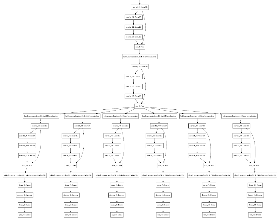
metrics=['accuracy'])[4] - 模型可视化. 基于 keras.utils 的 plot_model 工具.
plot_model(self.cnn_model, to_file='consolidated_model.png')[5] - 开始模型训练. 建议保留 callbacks 以保存最佳模型(或模型权重),以及添加 EarlyStopping 以避免过拟合以及不必要的计算.
def train_model(self,
                x_train, y_train,
                x_val, y_val,
                save_path,
                epochs=25,
                batch_size=16):
        #
        early_stopping = EarlyStopping(monitor='val_loss',
                                       min_delta=0,
                                       patience=5, verbose=1,
                                       mode='auto',
                                       restore_best_weights=True)
        #
        check_pointer = ModelCheckpoint(save_path,
                                        monitor='val_loss',
                                        verbose=1,
                                        save_best_only=True,
                                        save_weights_only=False,
                                        mode='auto', period=1)
        #
        history = self.cnn_model.fit(x_train, y_train,
                                    batch_size=batch_size,
                                    epochs=epochs,
                                    validation_data=(x_val, y_val),
                                    callbacks=[early_stopping,
                                               check_pointer])
        return history
对所有标签都具有较好表现的模型,依赖于问题的视觉复杂度. 因为卷积层(convolutional filters)被要求同时(联合)的学习所有标签的 ROI,任何表现较弱的标签都会对模型的性能有不利影响(相比于独立的CNN 分类器).
训练过程损失函数衰减和性能曲线如图,可以看出,某些属性的模型可以不用很深的网络即可获得相当不错的表现.
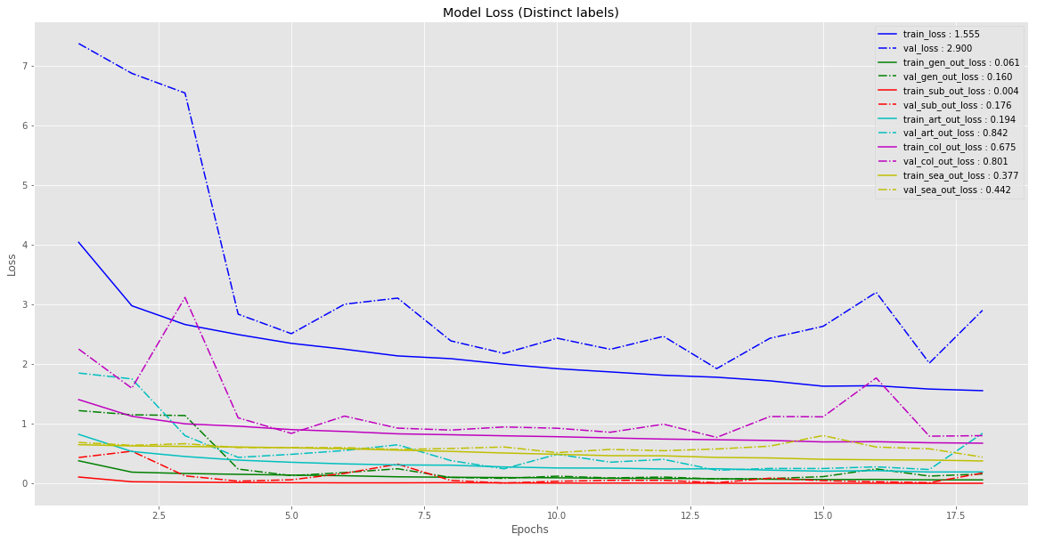
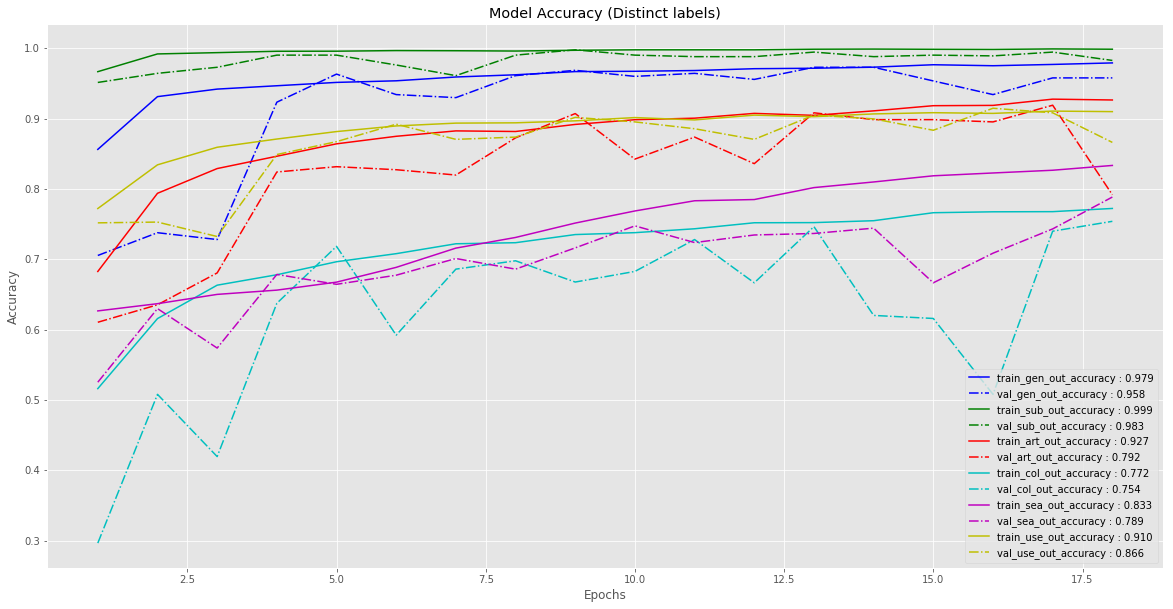
可以看出,对于某些标签,模型学习的相当快(尤其是对于类别较少的标签);而某些标签,比如颜色(color),模型就不能达到较优的性能(弱标注,weakly labelled). 总体而言,模型对于大部分标签取得了超过 95% 的精度.
3.1. 数据加载与处理实现
接 2.1.
# 选取部分数据,进一步分析
analysis_df = df.sample(frac=0.95, random_state=10)
analysis_df.reset_index(drop=True, inplace=True)

labels = analysis_df.keys()[1:-1].values
N = len(analysis_df)
print('Total nuber of Data_points {}\nLabels {}'.format(N, labels))
'''
Total nuber of Data_points 10269
Labels ['gender' 'subCategory' 'articleType' 'baseColour' 'season' 'usage']
'''

# 可视化,图片及其标签.
randm = np.random.randint(0, N)
img = mpimg.imread(analysis_df['img_path'][randm])

plt.figure(figsize=(7,7))
plt.imshow(img)
plt.title(str(analysis_df[labels].values[randm]))
plt.xlabel('Product_id :: {} \n Image shape :: {}'.format(
    str(analysis_df['id'][randm]), img.shape))
plt.show()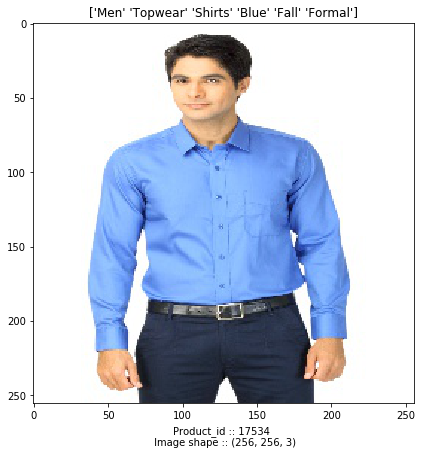
# 图片加载及预处理函数
def load_image(path, shape=(112,112,3)):
    image_list = np.zeros((len(path), shape[0], shape[1], shape[2]))
    for i, fig in enumerate(path):
        img = image.load_img(fig, color_mode='rgb', target_size=shape)
        x = image.img_to_array(img).astype('float16')
        x = x / 255.0
        image_list[i] = x
    return image_list


# 标签加载与处理
def load_attr(df, attr, N=None, det=False, one_hot=True):
    le = LabelEncoder()
    le.fit(df[attr])
    target = le.transform(df[attr])
    if N is None:
        N = len(set(target))
    if one_hot:
        target = to_categorical(target, num_classes=N)
    if det:
        print('\n{}:: \n{}'.format(attr,le.classes_))
        print('Target shape', target.shape)
    return le.classes_, N, target

# 数据分片
# 训练数据
x_train = load_image(analysis_df['img_path'][:t])

gen_names, num_gen, gender_tr = load_attr(analysis_df[:t], 'gender', det=True)
sub_names, num_sub, subCategory_tr = load_attr(analysis_df[:t], 'subCategory', det=True)
art_names, num_art, articleType_tr = load_attr(analysis_df[:t], 'articleType', det=True)
col_names, num_col, baseColour_tr = load_attr(analysis_df[:t], 'baseColour', det=True)
sea_names, num_sea, season_tr = load_attr(analysis_df[:t], 'season', det=True)
use_names, num_use, usage_tr = load_attr(analysis_df[:t], 'usage', det=True)

# 验证数据
x_val = load_image(analysis_df['img_path'][t:-100])

_, _, gender_val = load_attr(analysis_df[t:-100], 'gender', N=num_gen)
_, _, subCategory_val = load_attr(analysis_df[t:-100], 'subCategory', N=num_sub)
_, _, articleType_val = load_attr(analysis_df[t:-100], 'articleType', N=num_art)
_, _, baseColour_val = load_attr(analysis_df[t:-100], 'baseColour', N=num_col)
_, _, season_val = load_attr(analysis_df[t:-100], 'season', N=num_sea)
_, _, usage_val = load_attr(analysis_df[t:-100], 'usage', N=num_use)

# 后 100 张图片作为测试集
dict_ = {'gen_names' : gen_names.tolist(),
         'sub_names' : sub_names.tolist(),
         'art_names' : art_names.tolist(),
         'col_names' : col_names.tolist(),
         'sea_names' : sea_names.tolist(),
         'use_names' : use_names.tolist()}

json.dump(dict_, open('label_map.json', 'w'))
print('\n Distinct classes (Per label):',num_gen, num_sub, num_art, num_col, num_sea, num_use)
print('Shape:: Train: {}, Val: {}'.format(x_train.shape, x_val.shape))
输出如:
gender::
['Boys' 'Men' 'Women']
Target shape (9242, 3)

subCategory::
['Innerwear' 'Topwear']
Target shape (9242, 2)

articleType::
['Briefs' 'Kurtas' 'Shirts' 'Tops' 'Tshirts']
Target shape (9242, 5)

baseColour::
['Black' 'Blue' 'Green' 'Grey' 'Navy Blue' 'Purple' 'Red' 'White']
Target shape (9242, 8)

season::
['Fall' 'Summer']
Target shape (9242, 2)

usage::
['Casual' 'Ethnic' 'Formal' 'Sports']
Target shape (9242, 4)

 Distinct classes (Per label): 3 2 5 8 2 4
Shape:: Train: (9242, 112, 112, 3), Val: (927, 112, 112, 3)
3.2. 模型结构
class Classifier():
    '''
    Contains Multi-label Multi-class architecture

    ***Arguments***
    input_shape    :: Input shape, format : (img_rows, img_cols, channels), type='tuple'
    pre_model      :: Pretrained model file path, file extension : '.h5', type='str'

    ***Fuctions***
    build_model()  :: Define the CNN model (can be modified & tuned as per usecase)
    train_model()  :: Model Training (optimizers and metrics can be modified)
    eval_model()   :: Predict classes (in one-hot encoding)
    '''

    def __init__(self, input_shape=(112,112,3), pre_model=None):
        self.img_shape = input_shape

        # Load/Build Model
        if pre_model is None:
            self.cnn_model = self.build_model()
        else:
            try:
                self.cnn_model = load_model(pre_model)
            except OSError:
                print('Unable to load {}'.format(pre_model))

        # Compile Model
        self.cnn_model.compile(loss='categorical_crossentropy',
                               optimizer='adam',
                               metrics=['accuracy'])

        plot_model(self.cnn_model, to_file='consolidated_model.png')
        self.cnn_model.summary()


    def custom_residual_block(self, r, channels):
        r = BatchNormalization()(r)
        r = Conv2D(channels, (3, 3), activation='relu')(r)
        h = Conv2D(channels, (3, 3), padding='same', activation='relu')(r)
        h = Conv2D(channels, (3, 3), padding='same', activation='relu')(h)
        h = Conv2D(channels, (3, 3), padding='same', activation='relu')(h)
        return add([h, r])


    def build_model(self):
        input_layer = Input(shape=self.img_shape)

        # Conv Layers
        en_in = Conv2D(16, (5, 5), activation='relu')(input_layer)
        h = MaxPooling2D((3, 3))(en_in)

        h = self.custom_residual_block(h, 32)
        h = self.custom_residual_block(h, 32)

        h = self.custom_residual_block(h, 48)
        h = self.custom_residual_block(h, 48)

        h = self.custom_residual_block(h, 48)
        h = self.custom_residual_block(h, 48)

        h = self.custom_residual_block(h, 54)
        h = self.custom_residual_block(h, 54)
        en_out = self.custom_residual_block(h, 54)

        # Dense gender
        gen = self.custom_residual_block(en_out, 48)
        gen = GlobalAveragePooling2D()(gen)
        gen = Dense(100, activation='relu')(gen)
        gen = Dropout(0.1)(gen)
        gen = Dense(50, activation='relu')(gen)
        gen_out = Dense(num_gen, activation='softmax', name= 'gen_out')(gen)

        # Dense subCategory
        sub = self.custom_residual_block(en_out, 48)
        sub = GlobalAveragePooling2D()(sub)
        sub = Dense(100, activation='relu')(sub)
        sub = Dropout(0.1)(sub)
        sub = Dense(50, activation='relu')(sub)
        sub_out = Dense(num_sub, activation='softmax', name= 'sub_out')(sub)

        # Dense articleType
        art = self.custom_residual_block(en_out, 48)
        art = GlobalAveragePooling2D()(art)
        art = Dense(100, activation='relu')(art)
        art = Dropout(0.1)(art)
        art = Dense(50, activation='relu')(art)
        art_out = Dense(num_art, activation='softmax', name= 'art_out')(art)

        # Dense baseColour
        col = self.custom_residual_block(en_out, 48)
        col = GlobalAveragePooling2D()(col)
        col = Dense(100, activation='relu')(col)
        col = Dropout(0.1)(col)
        col = Dense(50, activation='relu')(col)
        col_out = Dense(num_col, activation='softmax', name= 'col_out')(col)

        # Dense season
        sea = self.custom_residual_block(en_out, 48)
        sea = GlobalAveragePooling2D()(sea)
        sea = Dense(100, activation='relu')(sea)
        sea = Dropout(0.1)(sea)
        sea = Dense(50, activation='relu')(sea)
        sea_out = Dense(num_sea, activation='softmax', name= 'sea_out')(sea)

        # Dense usage
        use = self.custom_residual_block(en_out, 48)
        use = GlobalAveragePooling2D()(use)
        use = Dense(100, activation='relu')(use)
        use = Dropout(0.1)(use)
        use = Dense(50, activation='relu')(use)
        use_out = Dense(num_use, activation='softmax', name='use_out')(use)

        return Model(input_layer, [gen_out, sub_out, art_out, col_out, sea_out, use_out])


    def train_model(self,
                    x_train, y_train,
                    x_val, y_val,
                    save_path,
                    epochs=25,
                    batch_size=16):
        #
        early_stopping = EarlyStopping(monitor='val_loss', min_delta=0,
                                       patience=5, verbose=1,
                                       mode='auto', restore_best_weights=True)
        #
        check_pointer = ModelCheckpoint(save_path, monitor='val_loss',
                                        verbose=1, save_best_only=True,
                                        save_weights_only=False,
                                        mode='auto', period=1)
        #
        history = self.cnn_model.fit(x_train, y_train,
                                    batch_size=batch_size,
                                    epochs=epochs,
                                    validation_data=(x_val, y_val),
                                    callbacks=[early_stopping, check_pointer])
        return history

    def eval_model(self, x_test):
        preds = self.cnn_model.predict(x_test)
        return preds
模型结构输出部分如:
3.3. 模型训练
ce = Classifier(pre_model=None)

history  = ce.train_model(x_train, [gender_tr, subCategory_tr, articleType_tr,
                                    baseColour_tr, season_tr, usage_tr],
                          x_val, [gender_val, subCategory_val, articleType_val,
                                  baseColour_val, season_val, usage_val],
                          save_path='consolidated_model.h5',
                          epochs=25,
                          batch_size=30)
3.4. 训练曲线可视化
 def learning_curves(hist):
        '''
        Learing curves included (losses and accuracies per label)
        '''
        plt.style.use('ggplot')

        epochs = range(1,len(hist['loss'])+1)
        colors = ['b', 'g' ,'r', 'c', 'm', 'y']

        loss_ = [s for s in hist.keys() if 'loss' in s and 'val' not in s]
        val_loss_ = [s for s in hist.keys() if 'loss' in s and 'val' in s]
        acc_ = [s for s in hist.keys() if 'acc' in s and 'val' not in s]
        val_acc_ = [s for s in hist.keys() if 'acc' in s and 'val' in s]

        # Loss (per label)
        plt.figure(1, figsize=(20,10))
        for tr, val ,c in zip(loss_, val_loss_, colors):
            plt.plot(epochs, hist[tr], c,
                     label='train_{} : {}'.format(tr, str(format(hist[tr][-1],'.3f'))))

            plt.plot(epochs, hist[val], '-.'+c,
                     label='{} : {}'.format(val, str(format(hist[val][-1],'.3f'))))

        plt.title('Model Loss (Distinct labels)')
        plt.xlabel('Epochs')
        plt.ylabel('Loss')
         plt.legend(loc='upper right')
        plt.show()

        # Accuracy (per label)
        plt.figure(2, figsize=(20,10))
        for tr, val, c in zip(acc_, val_acc_, colors):
            plt.plot(epochs, hist[tr], c,
                     label='train_{} : {}'.format(tr, str(format(hist[tr][-1],'.3f'))))

            plt.plot(epochs, hist[val], '-.'+c,
                     label='{} : {}'.format(val, str(format(hist[val][-1],'.3f'))))

        plt.title('Model Accuracy (Distinct labels)')
        plt.xlabel('Epochs')
        plt.ylabel('Accuracy')
        plt.legend(loc='lower right')
        plt.show()

learning_curves(history.history)
3.5. 预测
模型训练完成后,即可加载示例图片,并预测标签输出.
class Recognize_Item(object):
'''
Required:
image_path: path or url of the image file [Required]
model file: to be saved/updated at consolidated_model.h5
label_dict: to be saved/updated at label_map.json
'''
def __init__(self, model_path='consolidated_model.h5'):
self.model_path = model_path
def load_model(self):
'''
Load Consolidated model from utils
'''
try:
item_reco_model = load_model(self.model_path)
return item_reco_model
except Exception:
raise Exception('#-----Failed to load model file-----#')
def process_img(self, image_path):
'''
image: load & preprocess image file
'''
img = image.load_img(image_path, color_mode='rgb', target_size=(112,112,3))
x = image.img_to_array(img).astype('float32')
return x / 255.0
def tmp_fn(self, one_hot_labels):
'''
tmp function to manpulate all one-hot encoded values labels to --
-- a vector of predicted categories per labels
'''
flatten_labels = []
for i in range(len(one_hot_labels)):
flatten_labels.append(np.argmax(one_hot_labels[i], axis=-1)[0])
return self.class_map(flatten_labels)
def class_map(self, e):
'''
To convert class encoded values to actual label attributes
'''
label_map = json.load(open('label_map.json'))
dict_ = {'gen_names' : gen_names.tolist(),
'sub_names' : sub_names.tolist(),
'art_names' : art_names.tolist(),
'col_names' : col_names.tolist(),
'sea_names' : sea_names.tolist(),
'use_names' : use_names.tolist()}
gender = label_map['gen_names'][e[0]]
subCategory = label_map['sub_names'][e[1]]
articleType = label_map['art_names'][e[2]]
baseColour = label_map['col_names'][e[3]]
season = label_map['sea_names'][e[4]]
usage = label_map['use_names'][e[5]]
#
return [gender, subCategory, articleType, baseColour, season, usage]
def predict_all(self, model, image):
'''
Predict all labels
'''
x_image = np.expand_dims(image, axis=0)
return self.tmp_fn(model.predict(x_image))
def demo_results(self, image_path, ground_truth=None):
'''
To demo sample predictions
'''
image = self.process_img(image_path)
predicted_labels = self.predict_all(model, image)
#
plt.figure(figsize=(5,7))
plt.title('Fashion: Clothing Item recognition module')
plt.text(0, 133, str('Predictions : '+' | '.join(predicted_labels)),
fontsize=12, color='teal')
#
if ground_truth is None:
pass
else:
plt.text(0, 142, str('Ground Truth : '+' | '.join(ground_truth)),
fontsize=12, color='b')
#
plt.axis('off')
plt.imshow(image)
plt.show()
#
reco = Recognize_Item()
global model
model = reco.load_model()
# 预测和GT.
test_id = N-np.random.randint(0, 100)
reco.demo_results(analysis_df['img_path'][test_id],
ground_truth=analysis_df.ix[test_id,'gender':'usage'],)
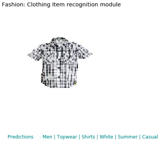
# 随机测试
test_id = N-np.random.randint(0, 100)
reco.demo_results(analysis_df['img_path'][test_id])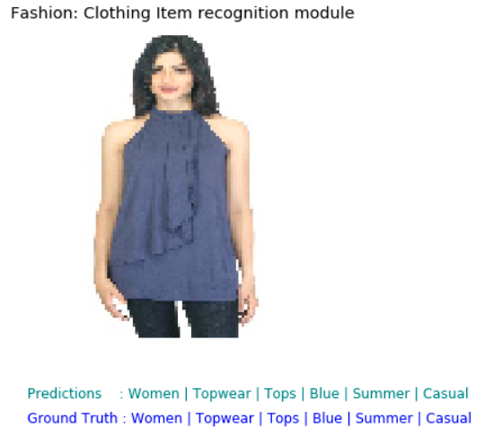
4. AWS 部署
可参考原文,基于 Flask、Docker、AWS 的部署.
1 条评论
您好,可以分享一下您的Docker吗?
最近有在学习视频结构化方面的东西,被困在多标签学习这一步了。