原文:Label smoothing with Keras, TensorFlow, and Deep Learning - 2019.12.30
这里主要介绍基于 Keras 和 TensorFlow 的标签平滑(lebel smoothing)实现的两种方式.
深度神经网络训练时,需要考虑两个重要的问题:
[1] - 训练数据是否过拟合;
[2] - 除了训练和测试数据集外,模型的泛化能力.
正则化方法被用于处理过拟合问题,提升模型的泛化能力. 比如,dropout,L2 Weight decay,数据增强, 等等.
不过,这里介绍另一种正则化技术 - 标签平滑.
标签平滑的特点有:
[1] - 将类别硬标签(hard class label)转化为软标签(soft label).
[2] - 直接对类别标签本身的操作.
[3] - 易于实现.
[4] - 可以提升模型的泛化能力.
首先,说明三个问题:
[1] - 什么是标签平滑
[2] - 标签平滑的作用
[3] - 为什么标签平滑能够提升输出模型的性能
此外,基于Keras 和 TensorFlow,给出两种标签平滑的实现:
[1] - 显式的对类别标签列表进行标签平滑.
[2] - 采用损失函数进行标签平滑.
1. 标签平滑以及其作用
在图像分类任务中,往往将类别标签进行硬性、二值处理(hard, binary assignments).
例如,MNIST 数据集的如下图片:

图中数字可以清晰的识别为 "7",其 one-hot 类别向量为:[0.0, 0.0, 0.0, 0.0, 0.0, 0.0, 0.0, 1.0, 0.0, 0.0].
这里硬标签编码:标签向量除了对应于数字 "7" 的第八个索引位置处的值为 1 以外,其他位置的元素均为 0.
而采用软标签编码的话,其 one-hot 类别向量类似于:[0.01 0.01 0.01 0.01 0.01 0.01 0.01 0.91 0.01 0.01].
其中,向量里的所有元素之和等于 1,类似于应标签编码向量.
软标签编码和硬标签编码的不同之处在于:
[1] - 硬编码的类别标签向量是二值的,如,一个类别标签是正类别,其他类别标签为负类别.
[2] - 软编码的类别标签中,正类别具有最大的概率;其他类别也具有非常小的概率.
为什么要这样做呢?
原因在于,不希望模型对其预测结果过度自信.
标签平滑可以降低模型的可信度,并防止模型下降到过拟合所出现的损失的深度裂缝里.
By applying label smoothing we can lessen the confidence of the model and prevent it from descending into deep crevices of the loss landscape where overfitting occurs.
2. 显式的类别标签平滑
实现如:
def smooth_labels(labels, factor=0.1):
    # smooth the labels
    labels *= (1 - factor)
    labels += (factor / labels.shape[1])

    # returned the smoothed labels
    return labels
以 CIFAR-10 数据集为例,基于 Keras 和 TensorFlow 的网络训练如:
# import the necessary packages
from pyimagesearch.learning_rate_schedulers import PolynomialDecay
from pyimagesearch.minigooglenet import MiniGoogLeNet
from sklearn.metrics import classification_report
from sklearn.preprocessing import LabelBinarizer
from tensorflow.keras.preprocessing.image import ImageDataGenerator
from tensorflow.keras.callbacks import LearningRateScheduler
from tensorflow.keras.optimizers import SGD
from tensorflow.keras.datasets import cifar10
import matplotlib.pyplot as plt
import numpy as np
import argparse


# construct the argument parse and parse the arguments
ap = argparse.ArgumentParser()
ap.add_argument("-s", "--smoothing", type=float, default=0.1,
    help="amount of label smoothing to be applied")
ap.add_argument("-p", "--plot", type=str, default="plot.png",
    help="path to output plot file")
args = vars(ap.parse_args())

# define the total number of epochs to train for initial learning
# rate, and batch size
NUM_EPOCHS = 70
INIT_LR = 5e-3
BATCH_SIZE = 64

# initialize the label names for the CIFAR-10 dataset
labelNames = ["airplane", "automobile", "bird", "cat", "deer", "dog",
    "frog", "horse", "ship", "truck"]

# 加载训练数据和测试数据;
# 并将图像从整数转换为 floats
print("[INFO] loading CIFAR-10 data...")
((trainX, trainY), (testX, testY)) = cifar10.load_data()
trainX = trainX.astype("float")
testX = testX.astype("float")

# 数据减均值
mean = np.mean(trainX, axis=0)
trainX -= mean
testX -= mean

# 将类别从整数转化为向量;
# 并将数据类型转换为 floats,以便进行标签平滑.
lb = LabelBinarizer()
trainY = lb.fit_transform(trainY)
testY = lb.transform(testY)
trainY = trainY.astype("float")
testY = testY.astype("float")

# 仅对训练数据类别标签进行标签平滑
print("[INFO] smoothing amount: {}".format(args["smoothing"]))
print("[INFO] before smoothing: {}".format(trainY[0]))
trainY = smooth_labels(trainY, args["smoothing"])
print("[INFO] after smoothing: {}".format(trainY[0]))

#construct the image generator for data augmentation
aug = ImageDataGenerator(
    width_shift_range=0.1,
    height_shift_range=0.1,
    horizontal_flip=True,
    fill_mode="nearest")

# construct the learning rate scheduler callback
schedule = PolynomialDecay(maxEpochs=NUM_EPOCHS, initAlpha=INIT_LR,
    power=1.0)
callbacks = [LearningRateScheduler(schedule)]

# initialize the optimizer and model
print("[INFO] compiling model...")
opt = SGD(lr=INIT_LR, momentum=0.9)
model = MiniGoogLeNet.build(width=32, height=32, depth=3, classes=10)
model.compile(loss="categorical_crossentropy", optimizer=opt,
    metrics=["accuracy"])

# 模型训练
print("[INFO] training network...")
H = model.fit_generator(
    aug.flow(trainX, trainY, batch_size=BATCH_SIZE),
    validation_data=(testX, testY),
    steps_per_epoch=len(trainX) // BATCH_SIZE,
    epochs=NUM_EPOCHS,
    callbacks=callbacks,
    verbose=1)

# 网络评估
print("[INFO] evaluating network...")
predictions = model.predict(testX, batch_size=BATCH_SIZE)
print(classification_report(testY.argmax(axis=1),
    predictions.argmax(axis=1), target_names=labelNames))

# construct a plot that plots and saves the training history
N = np.arange(0, NUM_EPOCHS)
plt.style.use("ggplot")
plt.figure()
plt.plot(N, H.history["loss"], label="train_loss")
plt.plot(N, H.history["val_loss"], label="val_loss")
plt.plot(N, H.history["accuracy"], label="train_acc")
plt.plot(N, H.history["val_accuracy"], label="val_acc")
plt.title("Training Loss and Accuracy")
plt.xlabel("Epoch #")
plt.ylabel("Loss/Accuracy")
plt.legend(loc="lower left")
plt.savefig(args["plot"])
3. 标签平滑损失函数
实现如:
# import the necessary packages
from pyimagesearch.learning_rate_schedulers import PolynomialDecay
from pyimagesearch.minigooglenet import MiniGoogLeNet
from sklearn.metrics import classification_report
from sklearn.preprocessing import LabelBinarizer
from tensorflow.keras.losses import CategoricalCrossentropy
from tensorflow.keras.preprocessing.image import ImageDataGenerator
from tensorflow.keras.callbacks import LearningRateScheduler
from tensorflow.keras.optimizers import SGD
from tensorflow.keras.datasets import cifar10
import matplotlib.pyplot as plt
import numpy as np
import argparse

# construct the argument parse and parse the arguments
ap = argparse.ArgumentParser()
ap.add_argument("-s", "--smoothing", type=float, default=0.1,
    help="amount of label smoothing to be applied")
ap.add_argument("-p", "--plot", type=str, default="plot.png",
    help="path to output plot file")
args = vars(ap.parse_args())

# define the total number of epochs to train for initial learning
# rate, and batch size
NUM_EPOCHS = 2
INIT_LR = 5e-3
BATCH_SIZE = 64

# initialize the label names for the CIFAR-10 dataset
labelNames = ["airplane", "automobile", "bird", "cat", "deer", "dog",
    "frog", "horse", "ship", "truck"]

#
print("[INFO] loading CIFAR-10 data...")
((trainX, trainY), (testX, testY)) = cifar10.load_data()
trainX = trainX.astype("float")
testX = testX.astype("float")

#
mean = np.mean(trainX, axis=0)
trainX -= mean
testX -= mean

# 将标签向量从整数转化为向量.
lb = LabelBinarizer()
trainY = lb.fit_transform(trainY)
testY = lb.transform(testY)

# construct the image generator for data augmentation
aug = ImageDataGenerator(
    width_shift_range=0.1,
    height_shift_range=0.1,
    horizontal_flip=True,
    fill_mode="nearest")

# construct the learning rate scheduler callback
schedule = PolynomialDecay(maxEpochs=NUM_EPOCHS, initAlpha=INIT_LR,
    power=1.0)
callbacks = [LearningRateScheduler(schedule)]

# initialize the optimizer and loss
print("[INFO] smoothing amount: {}".format(args["smoothing"]))
opt = SGD(lr=INIT_LR, momentum=0.9)
# 标签平滑损失函数
loss = CategoricalCrossentropy(label_smoothing=args["smoothing"])

print("[INFO] compiling model...")
model = MiniGoogLeNet.build(width=32, height=32, depth=3, classes=10)
model.compile(loss=loss, optimizer=opt, metrics=["accuracy"])

# train the network
print("[INFO] training network...")
H = model.fit_generator(
    aug.flow(trainX, trainY, batch_size=BATCH_SIZE),
    validation_data=(testX, testY),
    steps_per_epoch=len(trainX) // BATCH_SIZE,
    epochs=NUM_EPOCHS,
    callbacks=callbacks,
    verbose=1)

# evaluate the network
print("[INFO] evaluating network...")
predictions = model.predict(testX, batch_size=BATCH_SIZE)
print(classification_report(testY.argmax(axis=1),
    predictions.argmax(axis=1), target_names=labelNames))

# construct a plot that plots and saves the training history
N = np.arange(0, NUM_EPOCHS)
plt.style.use("ggplot")
plt.figure()
plt.plot(N, H.history["loss"], label="train_loss")
plt.plot(N, H.history["val_loss"], label="val_loss")
plt.plot(N, H.history["accuracy"], label="train_acc")
plt.plot(N, H.history["val_accuracy"], label="val_acc")
plt.title("Training Loss and Accuracy")
plt.xlabel("Epoch #")
plt.ylabel("Loss/Accuracy")
plt.legend(loc="lower left")
plt.savefig(args["plot"])
4. 训练过程曲线
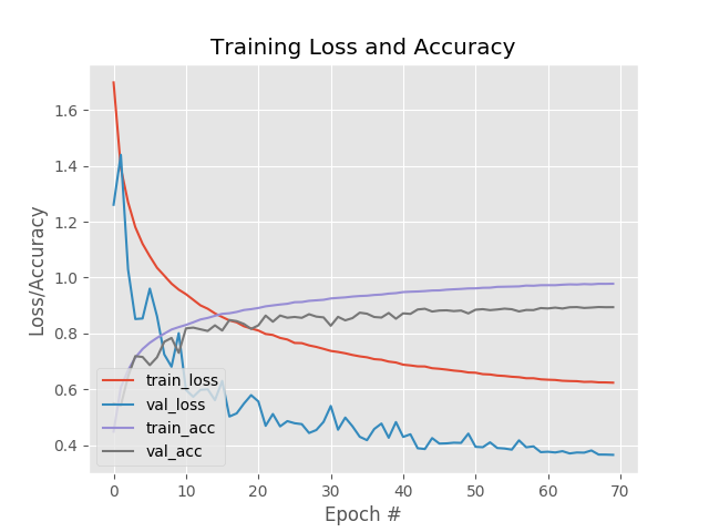
显式的类别标签平滑的训练过程曲线,如:
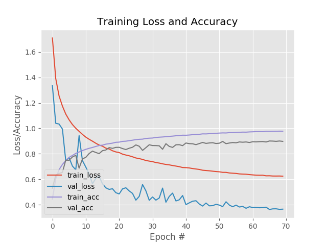
标签平滑损失函数的训练过程曲线,如:
5. 附 - 辅助函数
learning_rate_schedulers.py
import matplotlib.pyplot as plt
import numpy as np

class LearningRateDecay:
    def plot(self, epochs, title="Learning Rate Schedule"):
        # compute the set of learning rates for each corresponding
        # epoch
        lrs = [self(i) for i in epochs]

        # the learning rate schedule
        plt.style.use("ggplot")
        plt.figure()
        plt.plot(epochs, lrs)
        plt.title(title)
        plt.xlabel("Epoch #")
        plt.ylabel("Learning Rate")

class StepDecay(LearningRateDecay):
    def __init__(self, initAlpha=0.01, factor=0.25, dropEvery=10):
        # store the base initial learning rate, drop factor, and
        # epochs to drop every
        self.initAlpha = initAlpha
        self.factor = factor
        self.dropEvery = dropEvery

    def __call__(self, epoch):
        # compute the learning rate for the current epoch
        exp = np.floor((1 + epoch) / self.dropEvery)
        alpha = self.initAlpha * (self.factor ** exp)

        # return the learning rate
        return float(alpha)

class PolynomialDecay(LearningRateDecay):
    def __init__(self, maxEpochs=100, initAlpha=0.01, power=1.0):
        # store the maximum number of epochs, base learning rate,
        # and power of the polynomial
        self.maxEpochs = maxEpochs
        self.initAlpha = initAlpha
        self.power = power

    def __call__(self, epoch):
        # compute the new learning rate based on polynomial decay
        decay = (1 - (epoch / float(self.maxEpochs))) ** self.power
        alpha = self.initAlpha * decay

        # return the new learning rate
        return float(alpha)

if __name__ == "__main__":
    # plot a step-based decay which drops by a factor of 0.5 every
    # 25 epochs
    sd = StepDecay(initAlpha=0.01, factor=0.5, dropEvery=25)
    sd.plot(range(0, 100), title="Step-based Decay")
    plt.show()

    # plot a linear decay by using a power of 1
    pd = PolynomialDecay(power=1)
    pd.plot(range(0, 100), title="Linear Decay (p=1)")
    plt.show()

    # show a polynomial decay with a steeper drop by increasing the
    # power value
    pd = PolynomialDecay(power=5)
    pd.plot(range(0, 100), title="Polynomial Decay (p=5)")
    plt.show()
minigooglenet.py
from tensorflow.keras.layers import BatchNormalization
from tensorflow.keras.layers import Conv2D
from tensorflow.keras.layers import AveragePooling2D
from tensorflow.keras.layers import MaxPooling2D
from tensorflow.keras.layers import Activation
from tensorflow.keras.layers import Dropout
from tensorflow.keras.layers import Dense
from tensorflow.keras.layers import Flatten
from tensorflow.keras.layers import Input
from tensorflow.keras.models import Model
from tensorflow.keras.layers import concatenate
from tensorflow.keras import backend as K

class MiniGoogLeNet:
    @staticmethod
    def conv_module(x, K, kX, kY, stride, chanDim, padding="same"):
        # define a CONV => BN => RELU pattern
        x = Conv2D(K, (kX, kY), strides=stride, padding=padding)(x)
        x = BatchNormalization(axis=chanDim)(x)
        x = Activation("relu")(x)

        # return the block
        return x

    @staticmethod
    def inception_module(x, numK1x1, numK3x3, chanDim):
        # define two CONV modules, then concatenate across the
        # channel dimension
        conv_1x1 = MiniGoogLeNet.conv_module(x, numK1x1, 1, 1,
            (1, 1), chanDim)
        conv_3x3 = MiniGoogLeNet.conv_module(x, numK3x3, 3, 3,
            (1, 1), chanDim)
        x = concatenate([conv_1x1, conv_3x3], axis=chanDim)

        # return the block
        return x

    @staticmethod
    def downsample_module(x, K, chanDim):
        # define the CONV module and POOL, then concatenate
        # across the channel dimensions
        conv_3x3 = MiniGoogLeNet.conv_module(x, K, 3, 3, (2, 2),
            chanDim, padding="valid")
        pool = MaxPooling2D((3, 3), strides=(2, 2))(x)
        x = concatenate([conv_3x3, pool], axis=chanDim)

        # return the block
        return x

    @staticmethod
    def build(width, height, depth, classes):
        # initialize the input shape to be "channels last" and the
        # channels dimension itself
        inputShape = (height, width, depth)
        chanDim = -1

        # if we are using "channels first", update the input shape
        # and channels dimension
        if K.image_data_format() == "channels_first":
            inputShape = (depth, height, width)
            chanDim = 1

        # define the model input and first CONV module
        inputs = Input(shape=inputShape)
        x = MiniGoogLeNet.conv_module(inputs, 96, 3, 3, (1, 1),
            chanDim)

        # two Inception modules followed by a downsample module
        x = MiniGoogLeNet.inception_module(x, 32, 32, chanDim)
        x = MiniGoogLeNet.inception_module(x, 32, 48, chanDim)
        x = MiniGoogLeNet.downsample_module(x, 80, chanDim)

        # four Inception modules followed by a downsample module
        x = MiniGoogLeNet.inception_module(x, 112, 48, chanDim)
        x = MiniGoogLeNet.inception_module(x, 96, 64, chanDim)
        x = MiniGoogLeNet.inception_module(x, 80, 80, chanDim)
        x = MiniGoogLeNet.inception_module(x, 48, 96, chanDim)
        x = MiniGoogLeNet.downsample_module(x, 96, chanDim)

        # two Inception modules followed by global POOL and dropout
        x = MiniGoogLeNet.inception_module(x, 176, 160, chanDim)
        x = MiniGoogLeNet.inception_module(x, 176, 160, chanDim)
        x = AveragePooling2D((7, 7))(x)
        x = Dropout(0.5)(x)

        # softmax classifier
        x = Flatten()(x)
        x = Dense(classes)(x)
        x = Activation("softmax")(x)

        # create the model
        model = Model(inputs, x, name="googlenet")

        # return the constructed network architecture
        return model
6. 相关文献
[1] - Label Smoothing - 标签平滑理论推导
[2] - When Does Label Smoothing Help?
[3] - Bag of Tricks for Image Classification with Convolutional Neural Networks